Module 1 — Introduction to Machine Learning
1.1 Introductory Comments
Machine Learning (ML) is a vast and well-developed area that combines ideas from multiple fields. Toolkits like Scikit-learn, PyTorch, TensorFlow make it widely available. This course will be based on existing toolkits and will go over several algorithms and techniques. But perhaps more importantly, the course aims to present the intuition behind these algorithms, in order to make you better users of the toolkits, or even guide you to design your own Machine Learning algorithms.
We will develop this intuition about ML algorithms by reflecting about ourselves, as ML is sometimes an attempt at reverse-engineering our own learning processes. We will also need some mathematical tools, from linear algebra, calculus and probability. We will be introducing these notions smoothly, and only when needed. We will be working with Python at a level that does not require prior working knowledge of the language.
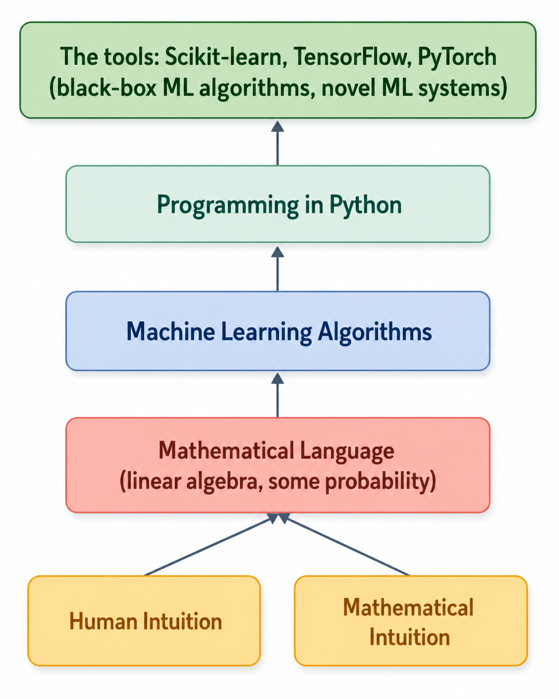
The chapters in these notes will be color-coded accordingly.
1.2 Supervised Learning ⬤ 
1.2.1 Classification
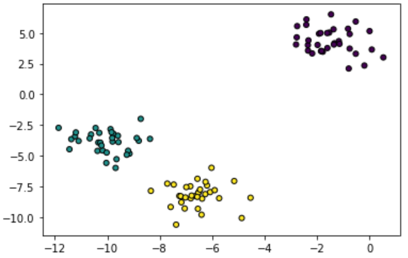
What we see in the following picture is a 2-dimensional dataset: each point $i$ has two coordinate attributes $(x_i,y_i)$. In addition, each point has a label which in the picture is shown as a different color. The moment we see this dataset we instictively come up with some hypothesis about what type of generative process produces these points. And based on that hypothesis we are able to generalize and infer the label of new points. For example, it is likely that we will infer that point $(-6,-10)$ would have a yellow label. That is, given the supervision information (i.e. the color labels), we are able to classify unseen points. This type of learning task is known as supervised classification.
1.2.2 Regression
We view the data in the following picture as a 1-dimensional dataset, where each point $i$ has a numerical attribute $x_i$. Of course, each point is also associated with a coordinate $y_i$, but we now view it as a numerical label for point $i$. Looking at this figure we likely now infer that there is an approximate linear relationship between $x_i$ and $y_i$, or perhaps a precise linear law that we observe slightly inaccurately, possibly due to measurement errors. Again, given some new point $x'$, we should be able to approximately infer a numerical label $y'$ for it. This type of learning task is known as regression.
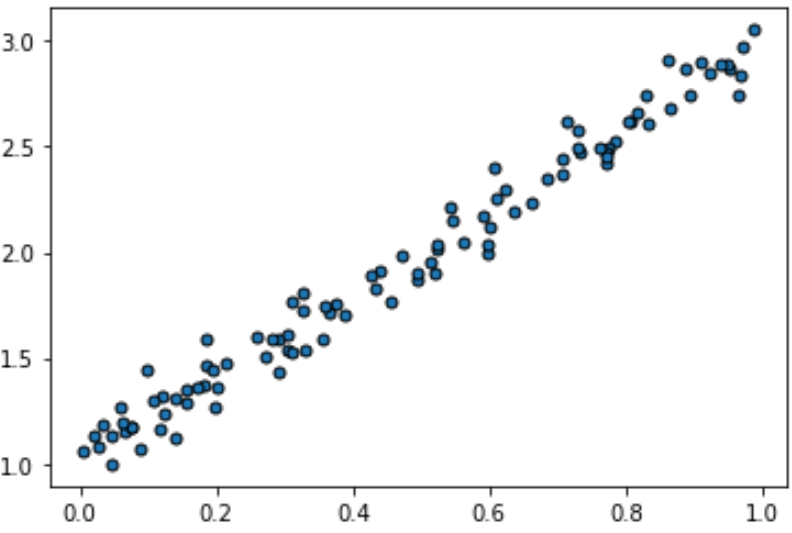
So, what differentiates classification from regression is what type of thing we try to predict: a categorical label, or a numerical label.
1.3 Data ⬤ 
The above 'toy' datasets follow simple geometric patterns and are easily visualizable in 2D plots. But the abstraction of data as geometric is vastly powerful. Almost all data can be viewed as, or transformed into, numerical points in some number of dimensions. A dataset can in fact have easily millions of dimensions. Let's see some examples.
The Iris flowers dataset
As an example, we can consider the 'Iris' dataset, that we will use frequently to demonstrate algorithms.
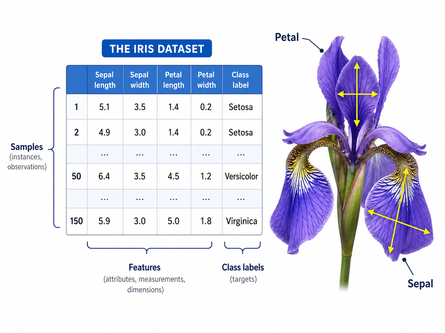
The dataset contains 150 points, and each point consists of four numerical coordinates, i.e. the dataset is 4-dimensional. Also, each point has a label, indicating one of three possible subspecies of the Iris flower. We see then how easy it is to have higher dimensional datasets, where visualization becomes impossible.
An image dataset
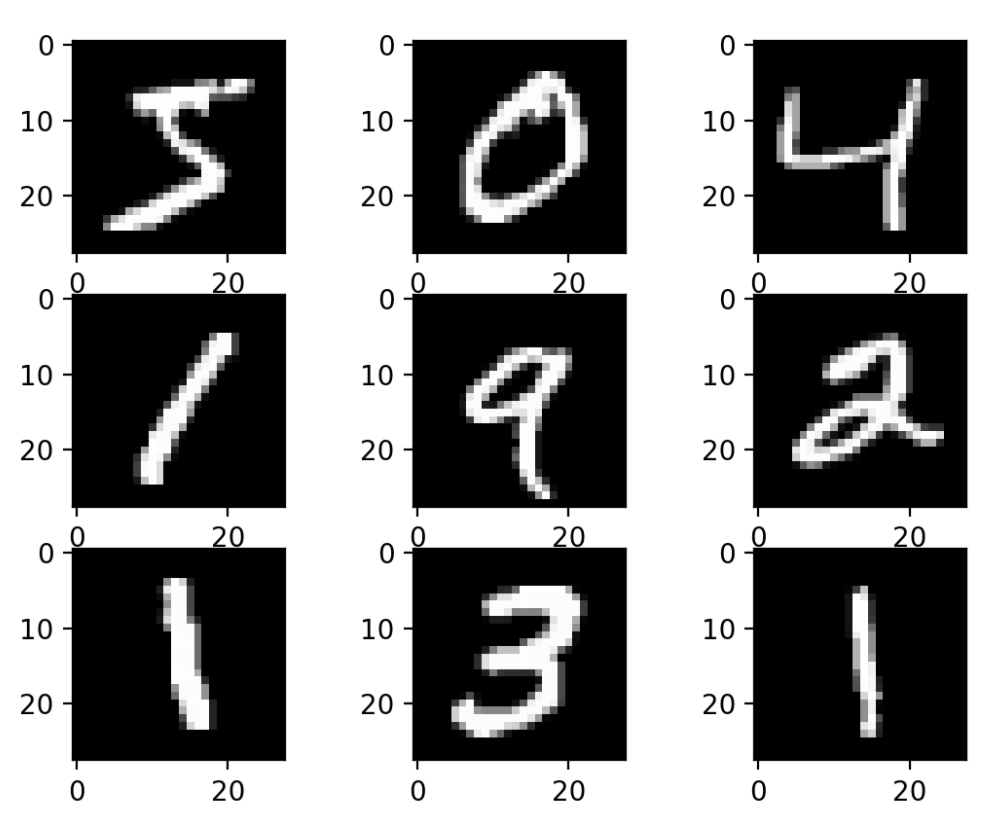
The above picture shows a dataset that consists of 9 images. While we can instantly perceive each image as a single entity, in fact each of these images is also a point: the 28x28 image consists of 784 pixels that we can order in some fixed way, e.g. row-wise. Each of these pixels can be viewed as a coordinate, and the numerical value of this coordinate will be a value in the range [0,255] indicating the 'greyness' of the pixel (with '0' being totally black, and '255' being totally white). So, this set of images can be viewed a 784-dimensional dataset! The number of dimensions can be much higher for larger images.
Higher-Dimensional Non-Visualizable Data
For the 784-dimensional image dataset, there is a 2D arrangement of the attributes that makes sense to us visually. But such arrangements do not exist in general.
Human brains are equipped with functions that allow us to very quickly handle visual information in 2 and 3 dimensions. Some people can mentally handle 4 dimensions, possibly by making analogies with 'time' as the 4th dimension. But in general, our ability to perceive and visualize data in 'higher' dimensions is extremely limited. That is one reason we resort to linear algebra; its generality allows us to handle data of all dimensions in a uniform mathematical way.
While we are not able to 'see' higher dimensional images, parts of our brain may be still running algorithms that manipulate vectors in higher dimensions. This is perhaps suggested by the fact that a machine learning technique/algorithm known as word2vec has mapped words (of English and later other languages) to vectors, and what is surprising is that algebraic operations on these vectors are meaningful from a linguistic point of view! Here is a related article:
https://www.datasciencecentral.com/profiles/blogs/the-word2vec-algorithm
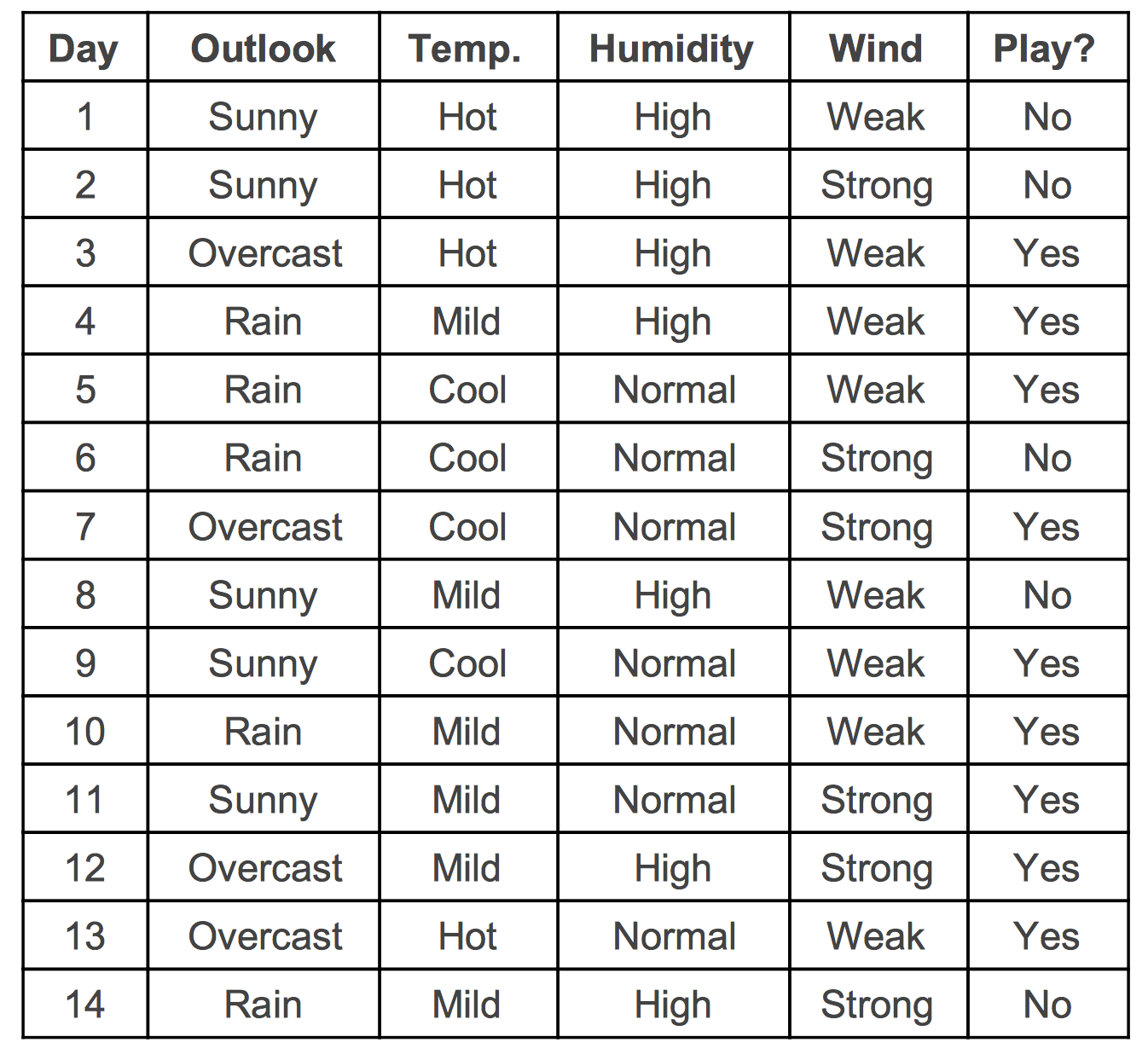
Non-numerical data
In the course we will also deal with datasets with categorical attributes, and machine learning algorithms that have been developed with such datasets in mind. Here is an example:
1.4 Data: Algebraic Notation ⬤ 
Linear Algebra is the mathematical language of Machine Learning. Here we introduce notation that will stick with us for the rest of the course. Let's do that via using the Iris Data set as an example.
In the given order of the data set, we will be denoting point $i$, as a row vector $x^{(i)}$ containing the four measurements of that point. For example, in the Iris data set, point 50 is:
$$x^{(50)} = [6.5, 3.5, 4.5, 1.2]$$
The entire data set can then be represented as an $n\times d$ matrix $X$, where row $i$ is a the vector corresponding to point $i$, and $d=4$ is the number of entries in each vector. In that sense we can view the data matrix $X$ as a column vector:
$$ \begin{align} y &= \begin{bmatrix} x^{(1)} \\ x^{(2)} \\ \vdots \\ x^{(n)} \end{bmatrix} \end{align} $$
The labels can also be represented as a column vector $y$ of integer numbers, where the numbers 0,1,2 are mapped to the three possible labels in some way.
1.5 Learning Bias ⬤ 
We are all familiar with learned bias, bias we acquire from data observation. For example the word 'dog' almost never evokes to you the picture of a 12ft tall animal accidentally slapping people with its tail. Learned bias is also encountered daily: some of us still think of a male when we hear of the word 'doctor', and that is precisely due to the data points we may have observed in the course of our daily lives. Bias is a serious problem in Machine Learning, and is a topic of active research.
On the other hand, there is also likely a learning bias, which we will later call the inductive bias, that we can think of as some type of mathematical constraint on how a machine learning algorithm operates. Such a mathematical constraint can be crucial to the ability of the algorithm to adapt and do well with natural data, but it also may be a source of occasional errors. We will make this more concrete in the context of ML, but a biological example may be illuminating: optical illusions.
Here is a binary (yes/no) classification problem for the following image: Are the diagonal lines parallel or not?

And, here is another one: is the following image moving or not?
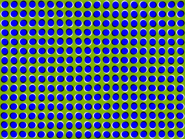
While we can be logically convinced about the true answers to the above questions, our visual classification algorithm seems to be compulsively making an error, and chances are that it is due to the architectural constraints of our visual system.
1.6 ML, DS and AI ⬤ 
Human brains apply their learned algorithms not only to basic every day tasks, but to more 'grand' goals, including understanding natural phenomena with the discovery of natural laws. For example Newton's law of gravity expresses the gravitational force $F$ between two masses $m_1$ and $m_2$ at distance $r$, as $$F = G\cdot \frac{m_1m_2}{r^2}.$$
Here $G$ is a parameter that we learned via measurements. This famous equation is nothing but a very special regression model, for 3D-data where the three coordinates are $[m_1,m_2,r]$.
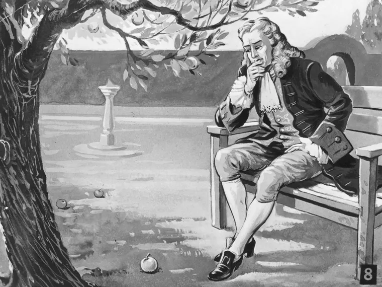
The iconic moment when Newton was inspired by the fallen apple was preceded by centuries of observation, measurement and thinking, and millenia of natural evolution, that resulted in human brains able to understand laws of nature.
It is likely that animals also partially understand basic natural laws [1]. And certainly evolution continues to 'experiment' with producing brains that are architecturally distinct and possible able to absorb natural data in different ways [2], [3].
Machine Learning is greatly hyped for its commercial applications. But perhaps more importantly, its recent achievements justify a speculation that ML constitutes the beginning of the 'post-theory' science [4] characterized by the theoryless understanding of complex natural phenomena via algorithmic devices that inherently possess 'learning biases' that extend those in our brains. Such devices are able to learn complex phenomena and successfully perform classification, regression, and other tasks on the associated complex data - in some sense, encoding a theory in a way that is opaque to humans. Such devices are designed by humans, but their discovery involves much research trial and error to produce the fittest algorithm, in a process that looks much like evolution. And while humans originally imagined Artificial Intelligence in an anthropomorphic way, perhaps AI will turn out to be an extension of human intelligence, and part of its natural evolution.
Plot generation code
The code in these cells was used to generate the plots in this module. They have been included for those who may be interested, but there is no need to run them.
# imports needed in the module

from IPython.display import Image
from IPython.display import Math
from IPython.display import Latex

import matplotlib.pyplot as plt
from sklearn.datasets import make_blobs
import numpy as np
X1, Y1 = make_blobs(n_features=2, centers=3, random_state = 1)
plt.scatter(X1[:, 0], X1[:, 1], marker="o", c=Y1, s=25, edgecolor="k")
<matplotlib.collections.PathCollection at 0x7b8d4985f190>

# Data Generation
np.random.seed(42)
x = np.random.rand(100, 1)
y = 1 + 2 * x + .1 * np.random.randn(100, 1)

# Shuffles the indices
idx = np.arange(100)
np.random.shuffle(idx)

plt.scatter(x,y, marker="o",  s=25, edgecolor="k")
<matplotlib.collections.PathCollection at 0x7b8d490923b0>
