Machine Learning Notes

Module 11 — Ensembles and Boosting

11.1 Society-Inspired Machine Learning ⬤

Human societies have learned to deal with very complex problems, using the synergy of multiple experts, even if individual experts understand only a small part of these problems. We make everyday use of many kinds of facilities that we often take for granted and even believe we understand, falling for the illusion of explanatory depth [1].

It is then not surprising that Machine Learning draws inspiration not just from biology, or from individual brains, but also from human and animal societies.

11.2 Simple Voting Ensembles ⬤

We have learned already about many different classifiers, with different inductive biases. A plausible hypothesis is that different inductive biases may lead to classifiers with different strengths for different types of inputs. Then a natural idea is to make an ensemble of different classifiers, where we combine their predictions for a point $x$ so as to produce a better and more reliable classification for $x$.

Suppose then that we have trained $N$ classifiers $C_1,\ldots,C_N$, for a classification problem with $c$ different classes. We can use these $N$ classifiers to make a prediction for $x$ as follows:

• Voting. Consider a point $x$ that receives a class label $y_i = C_i(x)$ from each classifier. A simple way to leverage these $N$ class predictions is to count which of the $c$ possible class labels comes up most often among the $N$ predictions, and return that label as the ensemble prediction. In case of a tie, we can split the tie arbitrarily.

• Voting by Probability / Confidence. In most cases, a classifier $C_i$ can return a vector $p^{(i)}_{j}$ of probabilities, where $p^{(i)}_{j}$ is the probability that point $x$ is in class $c_j$. We can compute a mean confidence for each label $c_j$: $$ m_j = \frac{1}{N}\sum_{i=1}^N p^{(i)}_{j} \, , $$ and select the class $j$ that has the highest mean $m_j$.

• Alternatively we can calculate the geometric mean for each label $C_j$ , $$ g_j = \bigg(\prod_{i=1}^N p^{(i)}_{j}\bigg)^{1/N} \, , $$ and again select the class $j$ that has the highest geometric mean $g_j$.

These N classifiers do not have to be all of the same kind, and obviously they can be trained independently from each other.

11.3 Bootstrapped Aggregation (Bagging) ⬤

In a society of human learners, the learning process is never perfect. Every individual can be trained only on a subset of the available knowledge — in other words, she observes only some of the available training points, and pays attention to only some of their features.

This observation underlies the intuition of a method of ensemble learning known as bagging, short for 'Bootstrapped AGgregation'.

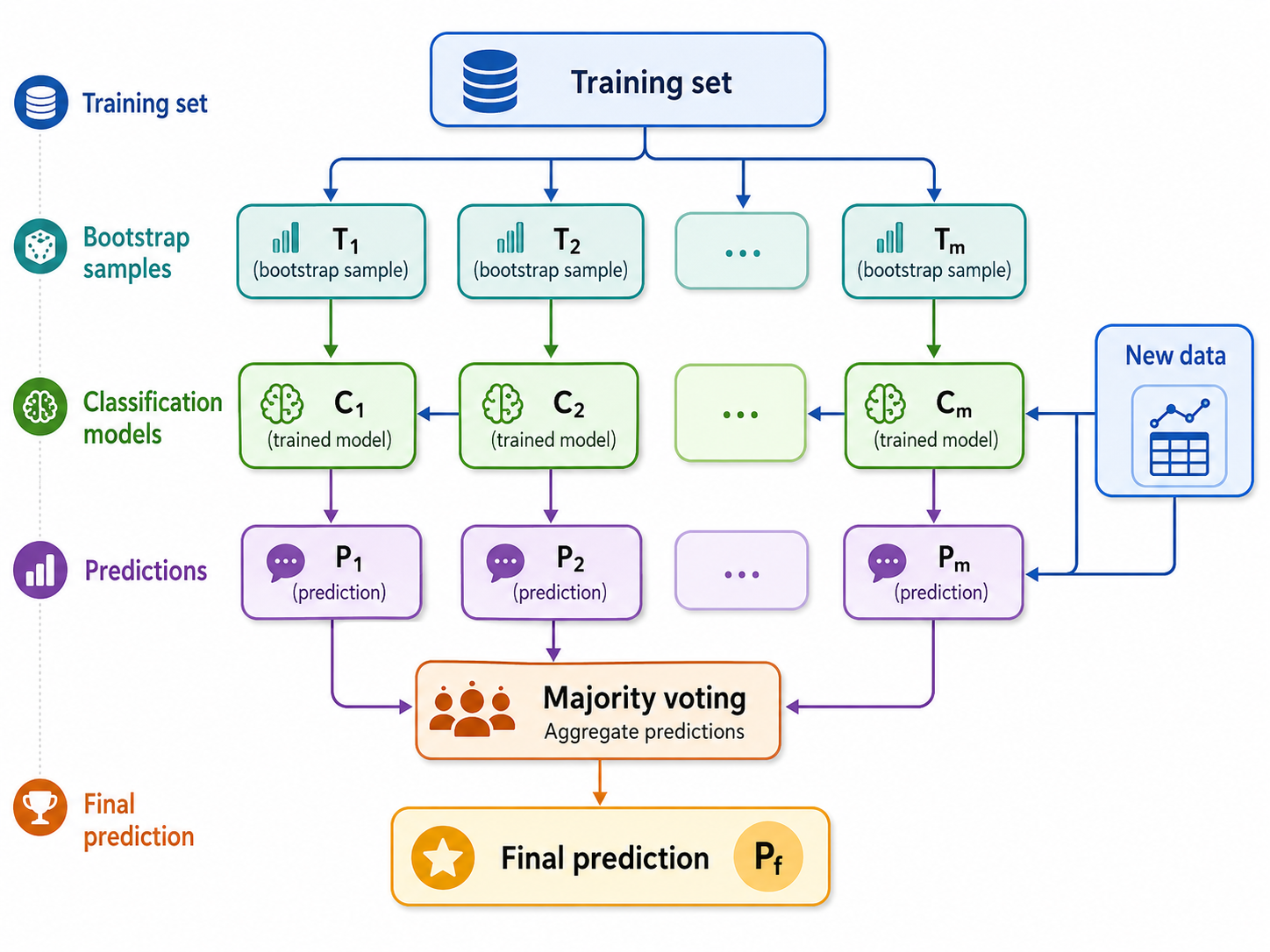
In bagging, we usually train classifiers of the same kind, although this is not strictly necessary. Here we train $m$ different classifiers. Each classifier randomly selects:

• $d'<d$ attributes, which together determine a submatrix of the data matrix $X$ consisting of $d'$ columns.

• $n'< n$ points (rows) from the data matrix $X'$, where each point can be picked more than once.

Then each classifier is trained with the dataset $X_i$ that it selected.

After having these $m$ classifiers trained, we can use the voting mechanisms we discussed in the previous section to classify a new point $x$.

Some points about bagging.

• Random Forests are a case of bagging applied to decision trees.
• While each classifier may overfit on its training set, the overall ensemble will likely generalize better, because it would be impossible for the majority of classifiers in the ensemble to overfit in the same way, and thus the different 'patterns of overfitting' will tend to cancel out. For that reason, when training a random forest, we typically let the decision trees grow longer, without caring so much about whether their questions become too narrow or specific.
• Similarly to the simple ensemble model we discussed in Section 11.2, the classifiers in a bagging ensemble can be trained independently and simultaneously, and in fact their training will be more efficient because their datasets will be smaller. Therefore, for the same amount of computation we can train bigger ensembles.

11.4 AdaBoost (Adaptive Boosting) ⬤

Unlike bagging that trains $N$ classifiers, Adaptive Boosting is an algorithm that is based on the idea of learning the classifiers $C_1,C_2,\ldots,C_N$ in a sequential order, in a way that 'forces' classifier $C_{i+1}$ to correct the mistakes of classifier $C_i$, by paying more attention to the training points that were misclassified by $C_i$. This is illustrated in the picture below.

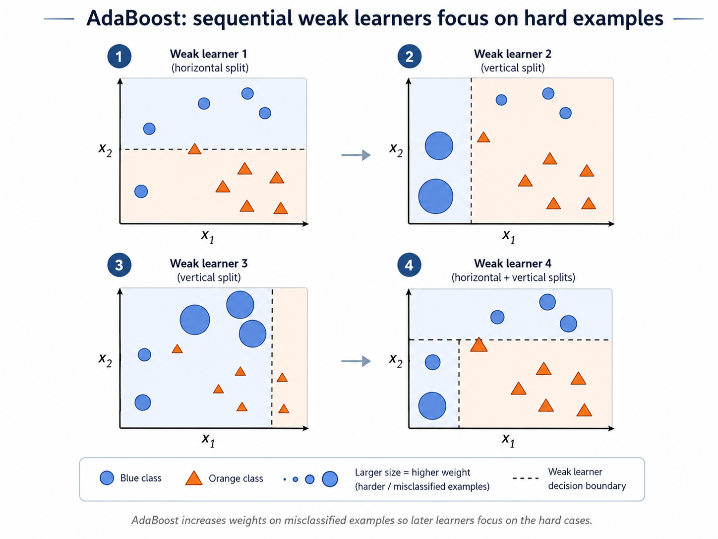
Naturally, this means that $C_{i+1}$ will be 'instructed' to overfit these points, and that can make its generalization worsen. For that reason we will give less voting power to classifier $C_{i+1}$. Then, assuming a good setting for the voting power of the classifiers, our ensemble will generalize better than each individual classifier.

11.4.1 Voting Weights

Until now, we have discussed ensembles where each of the classifiers is considered to be equally important, and so their votes (for a single class, or confidence/probabilities over classes) all received the same weight. However, with AdaBoost, we assign an importance weight $a_i$ to each classifier $C_i$, where $a_i>0$.

Given a point $x$, suppose that classifier $C_i$ issues a vector of probabilities $p^{(i)}$, where $p^{(i)}_j$ is the probability that point $x$ is in class $j$. We can then compute a weighted total confidence for each label $c_j$ , $$ m_j = \sum_{i=1}^N a_i p^{(i)}_j \, , $$

and select the class $j$ that gives the maximum weighted confidence $m_j$.

11.4.2 Weighted Loss Functions

Common loss functions are sums of the individual errors of the training points. For example, the negative log-likelihood function is $$ L = -\sum_{i=1}^n \left(y_i\log \hat{y}_i + (1-y_i)\log (1-\hat{y}_i)\right)\, , $$ where $y_i$ is the true 0/1 class label of point $X_i$, and $\hat{y}_i$ is a real-valued class prediction, expressed as a probability of $X_i$ being in class $1$.

This loss function gives the same importance weight to all individual points. However, we can define a more general loss function, where each point $X_i$ is associated with some importance weight $w_i>0$:

$$ L_{\mathit{weighted}} = -\sum_{i=1}^n w_i \left(y_i\log \hat{y}_i + (1-y_i)\log (1-\hat{y}_i)\right) \, . $$

Note: Sometimes it is convenient to consider that the importance weights $w_i$ sum up to $1$, in which case we will refer to them as normalized.

11.5 AdaBoost Pseudocode ⬤

The algorithm constructs an ensemble of $m$ binary classifiers, where $m$ is a hyperparameter. The dataset is $X$ and the training labels and the predictions are both assumed to be in $\{1,-1\}$.

• Initially, all $n$ points are given equal weights, $w^{({0})}_i$, for $i=1,\ldots n$.
• For $t=1,\ldots,m$ :
•     Train base classifier $b_t$ on $X$ with importance weights $w^{(t-1)}$.
•     Let $\epsilon_t$ be the training error of $b_t$ .
•     Calculate an importance weight for classifier $t$: $a_t = \frac{1}{2} \ln \frac{1-\epsilon_t}{\epsilon_t}$.
•     Update the weight of point $i$: $w_i^{(t)} = w_i^{(t-1)} e^{-a_t y_i b_t(X_i)}$.
•     Normalize the weights; i.e. let $S = \sum_{i=1}^n w_i$, and $w_i \leftarrow w_i/S$ .

In the end of this process we have $m$ binary classifiers, where classifier $C_t$ has importance $a_t$. We can then use these classifiers to make predictions on unseen points, as discussed in section 11.4.1.

Note 1: The importance weight for classifier $C_t$, $a_t = \frac{1}{2} \ln \frac{1-\epsilon_t}{\epsilon_t}$, is proportional to the log of the odds that the classifier is correct on a training point. In other words, the higher the training accuracy, the higher the voting weight of the classifier.

Note 2: If the classifier makes correct predictions more often than it makes mistakes (that is, if $\epsilon_t<0.5$), then the importance weight $a_t$ is positive. Otherwise, if mistakes are made more often than correct predictions, $a_t$ is actually negative!

Note 3: In the update formula for the weights, $b_t(X_i)$ is the label predicted for point $X_i$, and so $y_i b_t(X_i)$ can be either $1$ when the true and predicted labels are the same, or $-1$ otherwise. If classifier $b_t$ has a positive importance weight $a_t$, then when the true and predicted weights are different, the weight of point $i$ increases, and more attention will be given to it in the training of future classifiers. Otherwise, the weight decreases, and less attention will be given to it in future training. For classifiers that are "untrustworthy" ($a_t<0$), the effect on the importance weight of $X_i$ is reversed.

Note 4: AdaBoost requires that classifiers be trained sequentially, i.e. one at a time. However, when the ensemble is deployed, these classifiers can process the input independently, before their predictions are combined in the final voting step.

11.6 Gradient Boosting ⬤

Gradient Boosting is a more recent method for constructing ensembles of classifiers. One of its implementations (xgboost) has been widely used in Kaggle competitions, mostly by using boosted trees.

The basic idea behind gradient boosting is better understood in the context of regression. Suppose we have $n$ points and their numerical labels $(X_i,y_i)$ and we have learned some regression model $h_0$ that makes a prediction

$$ \hat{y}_i = h_0(X_i) \, . $$

Now, for every point $X_i$ we can calculate the residual error $r_i = y_i - \hat{y}_i$. If the first model can be improved, then it is likely the case that there will be some type of 'pattern' in these residuals. We can then try to add another model $h_1$ that will learn the residuals, i.e. design a regression model for the points $X_i$, with numerical labels $r_i$. The motivation is this: if we are able to learn a model $h_1$ such that $r_i = h_1(X_i)$, then we can completely correct the original model $h_0$, by using the 'composite' ensemble model:

$$ E(x) = h_0(x) + h_1(x) \, . $$

Of course, $h_1$ is not expected to be a fully perfect model for the regression problem $(X,r_i)$, so $E(x)$ will still have some residual error that we can try to model with yet another model $h_2$, and the process can continue in this way for a number of rounds $T$.

11.7 Ensembles and Boosting Notebook ⬤

Here is the code notebook.