Machine Learning Notes

Module 12 — A Probabilistic Perspective for ML Algorithms

12.1 A Review of Probability ⬤

12.1.1 Expectation and Variance

Suppose $Y$ is a random variable — that is, every time we observe $Y$ its value is randomly determined. Then, $E[Y]$ is the expected value of $Y$, or simply put, its expectation or its mean. You can think of this as taking the average of multiple random observations of $Y$.

The variance of $Y$ defines the expected (average) deviation of $Y$ from its expectation (average) $E[Y]$, and is defined as follows: $$ \mathit{Var}[Y] = E[(Y-E[Y])^2] = E[Y^2] - (E[Y])^2 \, . $$

12.1.2 Events and Joint Probability

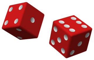
Imagine a die that has 6 faces as usual, but is biased — the faces do not have the same probability. Let's denote by $X$ the outcome of one die roll (a random variable). We assume that the probabilities of the 6 possible events for $X$ are given by this vector, denoted as $p_i = P(X=i)$. Here is the vector of probabilities we will consider:

$$p = \left[\frac{1}{12}, \frac{1}{12}, \frac{1}{3}, \frac{1}{6}, \frac{1}{6},\frac{1}{6}\right]\, .$$

This is what we call a discrete probability distribution, because there is a finite number of events, and the sum of their associated probabilities is equal to 1.

We also assume that the faces of the die are colored, and the colors are as follows:

[ red , blue , red , red , red , blue ]

For the experiment of rolling a die, we can then define another random variable $Y$ for the color of the outcome.

Joint Probability: The joint probability of two events is the probability that two events happen simultaneously. Some examples: $$ P(X = 1, Y = \mathit{red}) = 1/12\, , $$ and $$ P(X = 3, Y = \mathit{blue}) = 0 \, . $$

12.1.3 Conditional probability

Conditional Probability: We write $P(A|B)$ to denote the probability that event $A$ happens given that event $B$ happened. For example $P(Y = \mathit{red}\,|X=1)$ denotes the probability that the face is red given that it is 1, which we know is a certainty. So, we have $P(Y=\mathit{red}|X=1)=1$.

On the other hand, $P(X=1|Y = \mathit{red})$ denotes the probability that the dice roll is 1, given that we have already observed the color of the face (red). In that case, we have four different possible events of observing a red die face, but they do not have equal probabilities. The total probability of these four events is $9/12$ (the sum of the four probabilities), and the probability of $X=1$ is $1/12$.

$P(X=1|Y = \mathit{red}) = (1/12)/(9/12) = 1/9$.

(One intuitive way to think about this: in 120 statistically balanced rolls, 90 of them would be expected to have a red color, and among them 10 would also be $X=1$. So, the probability that we get $X=1$ is $1/9$.)

12.1.4 Marginalization

What is the probability that $Y=\mathit{blue}$? It would be tempting to say $1/3$, but that would be incorrect because the 6 faces are not equiprobable. In order to calculate it we will make use of marginalization:

$$P(Y=\mathit{blue}) = \sum_{i=1}^6 P(Y=\mathit{blue}\,|X=i)\,P(X=i)\, .$$

This expresses the probability of an event $Y$ based on the probabilities of the event conditioned on all possible outcomes of the second variable $X$. These conditional probabilities $P(Y|X=i)$ are weighted by the 'pure' probabilities $P(X=i)$.

We have $$ P(Y=\mathit{blue}) = 0*(1/12) + 1*(1/12) + 0*(1/3)+0*(1/6)+0*(1/6) + 1*(1/6) = 1/4\, . $$

We can see that this probability is smaller than $1/3$, and that is due to the one of the 'blue' events $X=1$ having a small probability.

12.1.5 Chain Rule for Probability

The chain rule for probabilities expresses the joint probability of two events as a product of two probabilities, one conditional and one unconditional. In general it looks like this:

$$P(A,B) = P(A|B)\,P(B)\, .$$

Let's see an example:

$$ P(X=2~\mathit{or}~X=3,Y = \mathit{blue}) = P(X=2~\mathit{or}~X=3\,|Y=\mathit{blue})\,P(Y=\mathit{blue}) \, . $$

We have already calculated $P(Y=blue)=1/4$. Now for $P(X=2~\mathit{or}~X=3\,|Y=\mathit{blue})$ we can see that this is equal to $P(X=2|Y=\mathit{blue})$ simply because $X=3$ is inconsistent with $Y=\mathit{blue}$. The total probability for the $X$ events when $Y=\mathit{blue}$ is $3/12$, so we have $P(X=2|Y=\mathit{blue}) = (1/12)/(3/12)=1/3$.

12.1.6 Probability Density Functions

So far we have been talking about discrete random variables with a finite number of possible outcomes. A random variable $X$ can be continuous, but since it would have an infinite number of possible outcomes, their 'individual' probability is 0. Instead we understand probability in terms of probability density functions $f(X)$ that can be used to tell us the probability that $X$ falls in a specific range of the continuum.

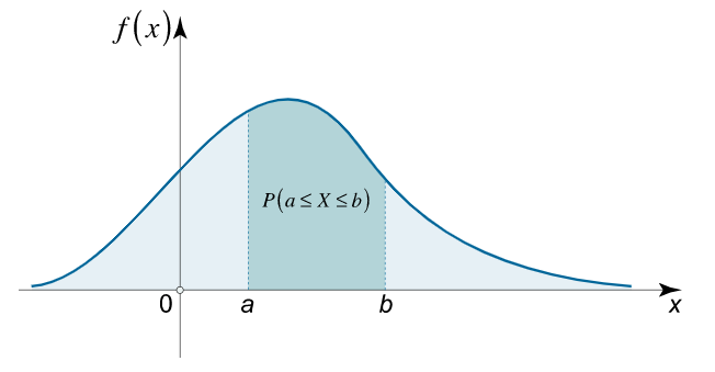
In the above example, the probability that $X$ is in the interval $[a,b]$ is equal to the area under the curve of $f(X)$, which is mathematically given by $$ \int_{a}^b f(x)\,\mathrm{d}x \, . $$

Most of the things we have discussed for discrete probabilities also transfer to the continuous case.

12.2 Error in Expectation ⬤

Supervised Machine Learning is based on the availability of training sets. These training sets are usually of a set of pairs of points and labels, of some finite fixed size: $$ D = \left\{(x_1,y_1), \ldots, (x_n,y_n) \right\} \, . $$

One way of thinking about data is to assume that they are produced by generative processes. In the simplest case, that could mean that there is a function $f$ for which we have $y_i = f(x_i)$. Our task in supervised ML is then to learn a model $\hat{f}$ such that $\hat{f}(x)$ is a good approximation for $f(x)$ — that is, $\hat{f}(x)$ has little error, not only on $D$, but also on other unseen points.

Let's assume that we have discovered a ML algorithm for which a "perfect" way of training it on a dataset $\cal D$ gives a model $\hat{f}$. Suppose $x$ is a fixed point. We can write $\hat{f}(x;D)$ to signify that the output of $\hat{f}$ does not depend only on the point $x$, but also on the dataset $D$ that we used to learn $\hat{f}$. Put simply, if $x$ is already part of $D$, then the error of $\hat{f}$ would be 0 on $x$ if the model were "perfectly" trained on $D$. However, if $x$ did not belong to $D$, the error can be far from zero. More generally, the error for $x$ would vary with the selection of $D$.

So, it makes sense to ask what the average error on $x$ would be, if taken over all possible selections of training set $D$. In a probabilistic sense, the error of $\hat{f}$ on point $x$ is a random variable that depends on the selection of the dataset $D$. We can then use the probabilistic notion of the expected squared error that we denote in this way:

$$ E_{D}\left[ \left(y - \hat{f}(x;D)\right)^2 \right] \, . $$

In this case the subscript in the expectation $E_{D}[\cdot]$ emphasizes the source of the randomness — the selection of the training set $D$.

12.3 Bias and Variance ⬤

Let's fix a point $x$.

Variance. We can define the variance of $\hat{f}(x;D)$ as follows: $$ \mathit{Var}_{D}\left[\hat{f}(x;D)\right] = E_{D}\left[ \left(E_{D}\left[\hat{f}(x;D)\right]- \hat{f}(x;D)\right)^2 \right] \, . $$

Let's parse this expression. Here we consider the random variable $Y = \hat{f}(x;D)$, i.e. the output of the model $\hat{f}$ under randomness in selecting the training set $D$. So, by definition, $\mathit{Var}_{D}\left[\hat{f}(x;D)\right] = \mathit{Var}\,(Y)$. The variance of the model measures how much the individual predictions on $x$ vary around the average prediction.

Bias. We also define:
$$ \mathit{Bias}_D\left[\hat{f}(x;D)\right] = E_D\left[\hat{f}(x;D)\right] - f(x) \, . $$

The bias shows how far the average of $\hat{f}(x;D)$ is from the 'true' $f(x)$. If that difference is large, then the algorithm and training process that gave $\hat{f}$ is 'biased' away from $f(x)$; that is, the inductive bias is too rigid and causes a significant error on $x$.

12.4 Bias and Variance Decomposition ⬤

Given these definitions, we can prove the following:

$$ E_{D}\left[ \left(y - \hat{f}(x;D)\right)^2 \right] = \left(\mathit{Bias}_{D}\left[\hat{f}(x;D)\right]\right)^2 + \mathit{Var}_D\left[\hat{f}(x;D)\right] . $$

In other words, across all choices of the training set $D$, the expected squared error for $\hat{f}$ is equal to the square of the model bias plus the model variance. In general, if the bias is high or the variance is high, then the expected squared error will be high.

The bias is a way of capturing 'underfitting', the tendency of the model to be wrong due to rigidity in its inductive bias. High bias leads to inaccurate predictions on average. On the other hand, high variance means that the model is too variable with respect to the choice of training sets D, which implies a capacity for 'overfitting'.

12.4.1 Adding Data Noise

Besides randomness in the selection of the training set $D$, we can also have randomness in the measured label. In particular, we may have $y = f(x)+\epsilon$, where $\epsilon$ is some random noise in the label. If we assume that $E[\epsilon] = 0$, and $\mathit{Var}[\epsilon] = \sigma^2$ (in the case when $y$ is just a scalar), then we have the following:

$$ E_{D,\epsilon}\left[ \left(y - \hat{f}(x;D)\right)^2 \right] = \left(\mathit{Bias}_{D}\left[\hat{f}(x;D)\right]\right)^2 + \mathit{Var}_D\left[\hat{f}(x;D)\right] + \sigma^2. $$

Here we see that the expectation also is taken over the second source of randomness (noise), and that under these assumptions, we obtain an additional term equal to the variance of the noise.

12.5 The Maximum Likelihood View ⬤

Example: Suppose $X$ is the height of a person, and $y$ is the event that their DNA contains a Y chromosome. We would like to predict the probability that a given $x$ corresponds to $y=1$ or $y=0$. In other words, we are looking for a way of estimating $P(y|x)$.

The notion of 'probability' here implies that there is an underlying generative random process that generates individuals, i.e. that there is a probability density function $f(x,y)$ for joint events $(x,y)$. This is an 'idealization' of reality that is common in Machine Learning and leads to interesting insights.

Our training set $D$ can contain data points $(x,y)$ that are drawn randomly from the existing distribution in the population. It is also a common assumption that these data are drawn from the same distribution $f(x,y)$, and they are drawn independently from one another. This 'identically and independently distributed' (iid) assumption is not necessarily an accurate one. For example, if our sample of individuals is not drawn from all areas of the world, then our $D$ may not reflect the 'true' distribution very well.

Nevertheless, we can assume both the existence of a generative process and iid data sampling.

12.5.1 Modeling with a Logistic Neuron

When we decide to train an algorithm on $D$, we are essentially making an assumption about the 'hidden law' that governs the data. Consider for example logistic regression. A logistic neuron is a model $m_w$ depending on parameters $w$ that takes as input a point $x$ and outputs a probability $m_w(X)$ that the label of $x$ is 1.

Our parametric model $m_w(x)$ is essentially a model for the probability distribution $P(y=1|x)$. Treating $P(y=1|x)$ as a model $m_w(x)$ imposes an inductive bias. But even if $m_w(x)$ can perfectly describe $P(y=1|x)$, we would still like to know the settings of the parameters $w$. But these parameters are determined through training on our dataset $D$. Since randomness has been used to sample $D$, we can assume that there is some probability that a specific setting for $w$ is correct.

All this means that we can reason in terms of a probability distribution $P(w|D)$. This can be a continuous probability density function, but since we do not have access to the generative process that gave $D$, this is a totally abstract notion. Still, if we wanted to pick the best parameters $w$, we would choose the setting that maximizes $P(w|D)$. Mathematically, this can be expressed as follows: $$ \hat{w} = \mathrm{argmax}_w~ P(w|D) \, . $$

Accessing $P(w|D)$ directly is impossible, but Bayes' Theorem comes to the rescue:

$$ P(w|D) = \frac{P(D|w)\,P(w)}{P(D)}. $$

Because $P(D)$ does not depend on the parameters $w$, we can ignore it, and solve the following problem instead: $$ \mathrm{argmax}_w~P(D|w)P(w) \, . $$

We can simplify the problem even further if there is no a priori probabilistic knowledge for any set of weights — that is, if any set of weights in our model is assumed to be equally probable. In this case, our problem becomes $$ \mathrm{argmax}_w~P(D|w) \, . $$

12.5.2 Deriving the NLL Loss

Suppose then that we have a dataset $D = \{(x_i,y_i)\}$ and a candidate model $m_w$. Because our problem is to model the probability that $y=1$ given $x$, we will view each point $(x_i,y_i)\in D$ as an observation of the random variable $y|x$, which takes values 1 or 0.

Because we have assumed that the data is independent, we have $$ P(D|w) = \prod_{i=1}^n P\left((y=y_i|x=x_i)|w\right) $$ If $y_i=1$, then $$P\left(\{y_i|x_i\}|w\right) = m_w(x_i)\, .$$ Otherwise, if $y_i=0$, $$P\left(\{y_i|x_i\}|w\right) = 1-m_w(x_i)\, .$$ This can be expressed in one equation as: $$ P\left(\{y_i|x_i\}|w\right) = m_w(x_i)^{y_i}\left(1-m_w(x_i)\right)^{1-y_i}\, . $$

We therefore want to solve the problem: $$ \mathrm{argmax}_w~P(D|w) = \mathrm{argmax}_w~ \prod_{i=1}^n m_w(x_i)^{y_i}(1-m_w(x_i))^{1-y_i}\, . $$ We can equivalently solve $$ \mathrm{argmax}_w~\log~P(D|w) \, , $$ in which case we get the log likelihood function, and looking for parameters for maximizing it. Alternatively, we can minimize the negative log likelihood (NLL) function.

So, our familiar NLL loss function can be viewed as a way of picking the parameters $w$ that are the most probable, given the data!

12.6 Naïve Bayes Classifier ⬤

We will now use the probabilistic approach to derive a simple classifier known as the Naïve Bayes Classifier. In this case we will assume that the input data is categorical.

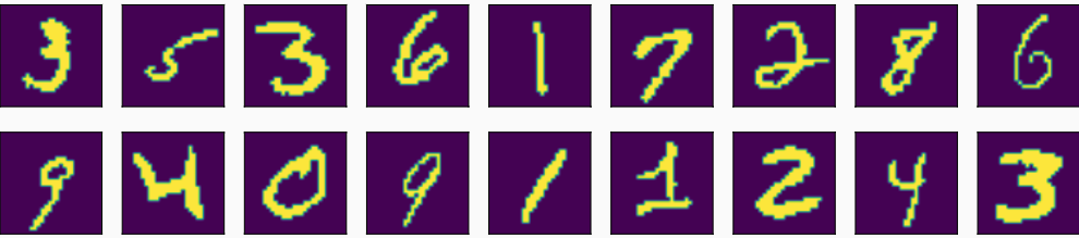
As an illustrative example, we will use the MNIST dataset. MNIST consists of 28x28 greyscale images, with each pixel represented by a number between 0 and 255. We will use a simplified version of MNIST, where the images are represented as a grid of pixels that are either 'black' (represented by 0) or 'white' (represented by 1). We can view each image as a vector of $28^2 = 784$ attributes, and all of them are 0 or 1.

These is how some of the images look like: they are single handwritten digits from 0 to 9. The dataset contains thousands of these images, and every image has a label from 0 to 9 corresponding to the digit it shows.

The probabilistic view assumes that there is a probability distribution $p(y|x)$ which assigns a probability to each label given the 784 attributes. Assuming we had access to $p(y|x)$, then the best decision we can make for a given input $x$ is this: $$ \hat{y} = \mathrm{argmax}_y\, p(y|x) \, . $$

However knowing or estimating $p(y|x)$ is extremely difficult, so Bayes' Theorem comes to the rescue again. We can instead solve the following problem:

$$ \hat{y} = \mathrm{argmax}_y\, \frac{p(x|y)p(y)}{p(x)} \, . $$

Again, since $p(x)$ does not involve $y$, we can solve the problem

$$ \hat{y} = \mathrm{argmax}_y\, p(x|y)p(y) \, . $$

We can now proceed with the estimation of $p(x|y)p(y)$ for each $y$.

Estimating $p(y)$: This is simply the probability that we observe label $y$ when we draw images from the distribution that generates them. In general we can use the training set $y$ for estimating that. For a given label $i$, we count the number of training points with label $i$, and divide by the total number of training points, and use this proportion as an estimate of $p(y=i)$.

Estimating $p(x|y)$: There are $2^{784}$ possible images, and $p(x|y)$ asks for the probability of each of them given the label $y$. This is an intractable calculation; however, we will work around this issue by assuming that the individual pixels are mutually independent (given the label). If $x_1,\ldots,x_{784}$ are the pixels of the image, independence implies that $$ p(x|y) = \prod_{t=1}^{784} p(x_t|y)\, . $$

We can estimate $p(x_t=i|y=j)$ as follows: We first count the number $n_j$ of the points where $y=j$. Then we count the number $s_i$ of points that have both $x_t=i$ and $y=j$. We can then use the estimate

$$p(x_t=i|y=j) = s_i\,/\,n_j\, .$$

This can be somewhat problematic because we can get $p(x_t = i)=0$, which would make $p(x|y)=0$. For that reason we use the so-called Laplace smoothing approximation for our estimate:

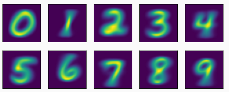
$$p(x_t=i|y=j) = \frac{s_i+1}{n_j+1}\, .$$

This assigns for each pixel $t$ a probability that it is black, given that the image has label $j$, for $j=0,\ldots,9$. These probabilities are visualized in the following picture where it can be seen that they recover nice smooth versions of the 10 digits!

We can then use these estimates to evaluate $p(x|y)$. In practice, since each class of MNIST has the same number of examples, each class label $y$ has the same probability $p(y)$. In such cases, it suffices to find the value $y$ that maximizes $p(x|y)$. Thus for MNIST we can instead solve the following equivalent problem:

$$ \hat{y} = \mathrm{argmax}_y \log p(x|y)p(y) = \mathrm{argmax}_y \log p(x|y) = \mathrm{argmax}_y \sum_{t=1}^{784} \log p(x_t|y)\, . $$