Module 13 — Dimensionality Reduction and Kernel PCA
In this module we will be looking at ways of transforming our dataset into a smaller yet (in some sense) equivalent dataset, so as to gain a benefit in the performance of learning models.
13.1 Introduction ⬤ 
Let $X$ be our dataset, represented as usual as an $n\times d$ matrix. A dimensional reduction of $X$ is a transformation to a new dataset $X'$ represented as an $n\times k$ matrix, for some $k$ that is smaller than $d$. Corresponding rows of $X$ and $X'$ refer to the same data objects, but their coordinate representations are typically very different.
Ideally, a good dimensional reduction should 'smooth out' the data while still preserving the relationships among the data to some degree, so that a task performed on $X'$ should have roughly the same outcome as if it had been performed on $X$. However, some information loss is to be expected. The smoothing of the data through dimensionality reduction can have the effect of reducing overfitting, leading to better prediction and better generalization.
Dimensionality reduction can be viewed as a form of data compression. The new format is more compact, and easier to work with. It allows for faster training of models, and faster search for hyperparameter settings.
Understanding dimensionality reduction requires some concepts in linear algebra. We will review this necessary background next.
13.2 Covariance ⬤ 
Dimensionality reduction involves finding a smaller number of attributes that can (more or less) do the same job as the original attribute set. Intuitively speaking, the greater the correlation among a group of attributes, the fewer features we would need to replace them. Here, we discuss a way of measuring how well or how poorly one attribute relates to another.
13.2.1 Variance and Covariance
We start with the familiar idea of variance. Given a list of values $$ a_1 = [a_{11}, a_{12}, \ldots, a_{1d}], $$ remember that its variance of $a_1$ is defined as the average squared deviation of the values of $a_1$ from its own average, $E[a_1]$: $$ \mathit{E}[a_1] \: = \: \frac{1}{d}\sum_{j=1}^d a_{1j} \, , \\ \mathit{Var}[a_1] \: = \: \frac{1}{d}\sum_{j=1}^d (a_{1j} - E[a_1])^2 \: = \: \frac{1}{d}\,(a_1 - E[a_1])\cdot (a_1 - E[a_1])^T \, . $$ The variance $\mathit{Var}[a_1]$ can be regarded as a standardized dot-product of the list $a_1$ with itself.
Now, instead of measuring the average squared deviation of values from their expectation within a single list, we can instead measure the average of the product of deviations of two different lists, $a_1$ and $a_2$. The population covariance is defined as follows: $$ \mathrm{Cov}[a_1,a_2] \: = \: \frac{1}{d}\sum_{j=1}^d (a_{1j} - \mathrm{E}[a_1])(a_{2j} - \mathrm{E}[a_2]) \: = \: \frac{1}{d}\,(a_1 - \mathrm{E}[a_1])\cdot (a_2 - \mathrm{E}[a_2]) \, , $$ or alternatively for samples: $$ \widehat{\mathrm{Cov}}[a_1,a_2] \: = \: \frac{1}{d-1}\sum_{j=1}^d (a_{1j} - \bar{a}_1)(a_{2j} - \bar{a}_2) \: = \: \frac{1}{d-1}\,(a_1 - \bar{a}_1 \mathbf{1})\cdot (a_2 - \bar{a}_2 \mathbf{1}) \, , $$ where $\bar{a}$ is the average of the entries of vector $a$, and $\mathbf{1}$ is the vector with all entries equal to $1$. The sample covariance $\widehat{\mathrm{Cov}}[a_1,a_2]$ can be regarded as a standardized dot-product of the lists $a_1$ and $a_2$.
In probabilistic terms, the covariance between two random variables $A$ and $B$ is given by $$ \mathit{Cov}[A,B] \: = \: E\left[(A-E[A])(B-E[B])\right] \, , $$ where $E[A]$ and $E[B]$ are the mathematical expectations of $A$ and $B$.
The covariance can be interpreted as a measure of the correlation between $A$ and $B$. The correlation is strongest when the magnitude of the covariance is largest. Note that unlike the variance, the covariance can be negative (in which case $A$ and $B$ are inversely correlated). When the covariance is zero, $A$ and $B$ are uncorrelated. This can happen when one of $A$ or $B$ is generated randomly and independently of the other.
13.2.2 Covariance Matrix
Let's return now to our $n\times d$ matrix $X$: $$ X = \left( \begin{array}{cccc} x_{11} & x_{12} & \cdots & x_{1d} \\ x_{21} & x_{22} & \cdots & x_{2d} \\ \vdots & \vdots & & \vdots \\ x_{n1} & x_{n2} & \cdots & x_{nd} \\ \end{array} \right) \, . $$
If we take the matrix product $X^T X$, we get something very special. The dimensions of the matrices are $d\times n$ and $n\times d$ (respectively), which means that the product matrix has dimensions $d\times d$. The $ij$-th entry of $X^T X$ is the product of the $i$-th row of $X^T$ and the $j$-column of $X$ — which is the same as the product of the $i$-th column of $X$ and the $j$-th column of $X$: $$ C_{ij} \: = \: \left(X^T X\right)_{ij} \: = \: \sum_{k=1}^n x_{ki}x_{kj} \: = \: a_i \cdot a_j \, , $$ where $a_i$ and $a_j$ are the $i$-th and $j$-th column vectors of $X$.
This means that if each entry of $X$ has been appropriately standardized by subtracting the average value over its attribute column, its column vector averages will all be zero (check it and see!). For such standardized matrices, the $ij$-th entry of $X^T X$ is simply $$ C_{ij} \: = \: a_i\cdot a_j \: = \: (a_i - E[a_i])\cdot (a_j - E[a_j]) \: = \: n\cdot\mathrm{Cov}[a_i,a_j] \, , $$ which is the covariance between column $a_i$ and column $a_j$ (times a constant factor $n$). For this reason, assuming that $X$ has been standardized in this way, $X^T X$ is called the covariance matrix of $X$.
13.3 Eigenvalues and Eigenvectors ⬤ 
The next important concept we will need from linear algebra concerns the special directions determined by a square transformation matrix.

13.3.1 Definition
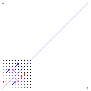
Imagine that we have the following $2\times 2$ square matrix. $$ A = \left[ \begin{array}{rr} 2 & 1 \\ 1 & 2 \\ \end{array} \right] \, . $$ Whenever a vector $w$ is multiplied by $A$, the result $Aw$ is a transformation of $w$ within the same $2$-dimensional space.
Usually the result of the transformation is a new vector with a different length, pointing in a new direction. However, for some vectors $w$, the transformed vector $Aw$ can lie in the same direction as $w$ (although the length could be different).
For example, if $w = [1, 1]^T$, the product is $$ Aw = \left[ \begin{array}{rr} 2 & 1 \\ 1 & 2 \\ \end{array} \right] \left[ \begin{array}{r} 1 \\ 1 \\ \end{array} \right] = \left[ \begin{array}{r} 3 \\ 3 \\ \end{array} \right] = 3\cdot \left[ \begin{array}{r} 1 \\ 1 \\ \end{array} \right] \, , $$ and if $w = [1, -1]^T$, the product is $$ Aw = \left[ \begin{array}{rr} 2 & 1 \\ 1 & 2 \\ \end{array} \right] \left[ \begin{array}{r} 1 \\ -1 \\ \end{array} \right] = \left[ \begin{array}{r} 1 \\ -1 \\ \end{array} \right] = 1\cdot \left[ \begin{array}{r} 1 \\ -1 \\ \end{array} \right] \, . $$ In general, vectors with the property that $Aw = \lambda w$ for some 'stretch' factor $\lambda$ are called eigenvectors of $A$. (The word eigen has its roots in German and Dutch, where one of its meanings is "own" or "self".) The factor $\lambda$ is the associated eigenvalue of $A$. In general, $A$ can be of any dimension $d\times d$.
The images above show the effect of a shear transformation on Leonardo da Vinci's Mona Lisa. The red vector is not an eigenvector, but the blue vector is (with eigenvalue 1).
The animation below shows the effect of the transformation $A$ on some vectors. Here, the directions of the blue and pink vectors are unchanged (eigenvectors), but the directions of the red vectors do change (not eigenvectors). Note that the blue vectors are stretched by a factor of 3 (eigenvalue = 3), while the length of the pink vectors is unaffected (eigenvalue = 1).
13.3.2 Some Properties of Eigenvectors
Eigenvectors and eigenvalues have many surprising and useful properties. We survey a few of them here. For the following, let us assume that matrix $A$ has eigenvectors $e_1, e_2, e_3, \ldots$ with corresponding eigenvalues $\lambda_1, \lambda_2, \lambda_3, \ldots$. Here, we also assume that these eigenvectors are distinct, in that they all have different directions.
13.3.2.1 Scaling
If $e_i$ is an eigenvector, then so is $ce_i$ for any non-zero real value $c$.
We can see this by letting $e'_i = ce_i$ and multiplying it by $A$: $$ Ae'_i = A(ce_i) = cAe_i = c\lambda_i e_i = \lambda_i (ce_i) = \lambda_i e'_i \, . $$
So, not only is $e'_i$ an eigenvector, it also has the same eigenvalue as $e_i$. Since all eigenvectors sharing the same direction also share the same eigenvalue, it is often convenient to assume that the eigenvectors are normalized to unit length (that is, scaled so that $\|e_i\|_2=1$).
13.3.2.2 Orthogonality
If the matrix $A$ is symmetric (that is, if $A^T = A$), then any pair of eigenvectors with distinct eigenvalues is orthogonal — that is, the pair of vectors forms a right angle, and their dot product is zero: $$ \lambda_i \neq \lambda_j \Longrightarrow e_i \cdot e_j = 0. $$
Verifying this on our example, we see that the matrix $A$ is indeed symmetric, since $a_{ij} = a_{ji}$ for every choice $i,j\in\{1,2\}$. Its two eigenvectors $e_1=[1,1]^T$ and $e_2=[1,-1]^T$ do have dot product $e_1\cdot e_2= (1)(1)+(1)(-1) = 0$. The orthogonality of $e_1$ and $e_2$ can also be seen in the animation above.
A nice property of covariance matrices is that they are always symmetric. To check this, we can take the transpose of $X^T X$ and observe that we get back the original matrix, $X^T X$: $$ (X^T X)^T = X^T (X^T)^T = X^T X \, . $$ The eigenvectors of a covariance matrix are therefore guaranteed to be mutually orthogonal.
13.3.2.3 Eigenvalues and the Frobenius Norm
Given a symmetric real-valued $d\times d$ matrix $A$, it is known that $A$ has an orthonormal basis of $d$ eigenvectors.
An interesting relationship exists between the entries of a matrix and its eigenvalues. If each entry $a_{ij}$ is squared and then added up, the total equals the sum of square of the eigenvalues. $$ \sum_{i=1}^d \sum_{j=1}^d a^2_{ij} = \sum_{i=1}^d \lambda^2_i \, . $$ The expression on the left is the square of a well-known norm for matrices, called the Frobenius norm. For an $n\times d$ matrix $X$, the Frobenius norm is $$ \|X\|_F = \sqrt{\sum_{i=1}^n \sum_{j=1}^d x^2_{ij}} \, . $$
13.3.3 Basis Vectors: A Review
Consider a column vector in 3D and how we can decompose it in terms of the 3 'basis' vectors, as follows:
$$ z = \left( \begin{array}{r} 3 \\ -2 \\ 5 \end{array} \right) = 3 \cdot \left( \begin{array}{r} 1 \\ 0 \\ 0 \end{array} \right) - 2 \cdot \left( \begin{array}{r} 0 \\ 1 \\ 0 \end{array} \right) + 5 \cdot \left( \begin{array}{r} 0 \\ 0 \\ 1 \end{array} \right) \, . $$
For simplicity, let's use the symbols $b_1,b_2,b_3$ for the 3 basis vectors. So we have
$$ z = \left( \begin{array}{r} 3 \\ -2 \\ 5 \end{array} \right) = 3 b_1 - 2 b_2 + 5 b_3 $$
Check any of these basis vectors, let's say $b_1$. We have $b_1^T b_1 = \|b_1\|_2^2 = 1$, which is telling us that the vector has length 1.
Now let's consider the inner (dot) product of a pair, e.g. $b_2,b_3$. We have $b_2^T b_3 = 0$. This means that the two vectors are orthogonal.
More generally, if we have two vectors $u,v$, then the inner product $u^T v$ is equal to $$ u^T v = \|u\|_2 \|v\|_2 \cos(\theta_{uv}) \, , $$ where $\theta_{uv}$ is the angle between $u$ and $v$. So, if both $u$ and $v$ have length $1$, then $u^T v$ is exactly equal to the cosine of their angle.
Consider now what happens when we take the inner product of our vector $z$, with say $b_1$.
$$
b_1^T z =
b_1^T \left( \begin{array}{r}
3 \\ -1 \\ 5
\end{array} \right) = b_1^T(3 b_1 - 2 b_2 + 5 b_3) = 3 b_1^T b_1 - 2 b_1^T b_2 + 5 b_1^T b_3 = 3
\, .
$$
In the last equality we used the fact that $b_1$ has length 1, and that it is orthogonal to the other two vectors. So, by performing this operation with $b_1$, we obtain a scalar which happens to be the coordinate of $b_1$ in the vector's decomposition!
This scalar, 3, is precisely the size of the projection of the vector $z$ to the direction of $b_1$. In a similar way we can compute the projections to $b_2$ and $b_3$.
13.3.4 Principal Components and Eigenvectors
Often, when we look for a dimensionality reduction for a data matrix $X$, we look for an alternative basis representation for $X$, with fewer basis vectors. In the principal component analysis (PCA) method, an alternative basis is obtained by computing the eigenvectors of the covariance matrix $C = X^T X$. This matrix $C$ is special, because it has an obvious product form, which among other things means that it is symmetric (i.e. $C_{ij} = C_{ji}$). Because $C$ has this special form, the eigenvalues are all positive, and more importantly, the eigenvectors are all orthogonal to each other.
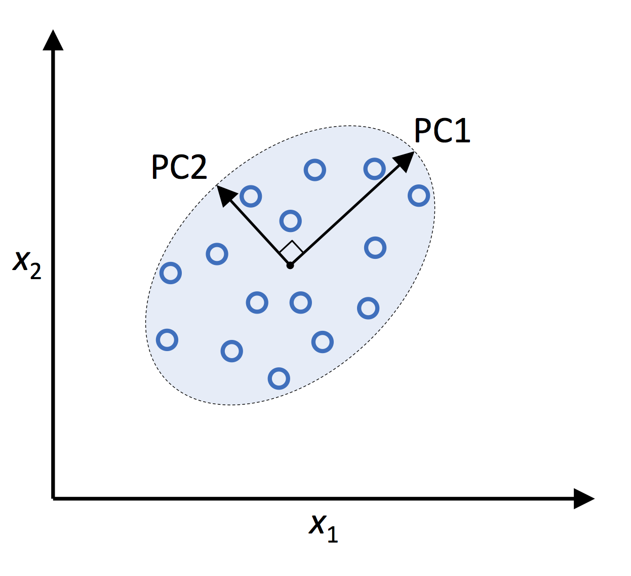
In the figure above, the two eigenvectors are orthogonal to each other, and so we can view them as alternative axes, that are essentially a transformation (in space) of the two standard axes.
As a simple example, suppose then that we have a 3D matrix $Z$, and that we have its three eigenvectors $e_1,e_2,e_3$, sorted in decreasing order of their eigenvalues (that is, with largest eigenvalues first). We know that any vector $z$ can be expressed in terms of $e_1$, $e_2$ and $e_3$ as a basis:
$$ z = \alpha_1 e_1 + \alpha_2 e_2 + \alpha_3 e_3 \, . $$
These constants $\alpha_1,\alpha_2,\alpha_3$ are the vector's coordinates in the alternative system of axes. The new basis vectors, these eigenvectors of $Z$, are referred to the principal components. The components are ordered, with the first principle component being the eigenvector with the largest eigenvalue.
While we still have $z$ expressed in its original coordinates, we can easily find its coordinates in the new system. For example we can find $\alpha_1$ as follows:
$$ e_1^T z = e_1^T (\alpha_1 e_1 + \alpha_2 e_2 + \alpha_3 e_3 ) = \alpha_1 e_1^T e_1 + \alpha_2 e_1^T e_2 + \alpha_3 e_1^T e_3 = 1\alpha_1 + 0\alpha_2 + 0\alpha_3 = \alpha_1 \, $$ or more generally, $$\alpha_i = e_i^T z \, .$$ Here we used again the fact that $e_1$, $e_2$, and $e_3$ form an orthogonal basis.
So, $\alpha_i = e_i^Tz = z^Te_i$ is exactly the size of the projection of $z$ onto the direction of principal component vector $e_i$.
Suppose now we make an $n \times 1$ vector $\alpha$ with all the projections of our data points onto the vector $e_i$, i.e.
$$ \alpha^{(i)} = \left( \begin{array}{c} a_1 \\ a_2 \\ \vdots \\ a_n \end{array} \right) $$
Then, we can express all projections succinctly, as
$$ \alpha^{(i)} = X e_i \, . $$
13.4 Principal Component Analysis (PCA) ⬤ 
Now that we have been introduced to eigenvectors and some of their properties, we are now ready to describe a strategy for dimensionality reduction, whereby we generate a transform of a dataset $X$ to some lower-dimensional setting. The PCA strategy involves creating a new basis for the data representation of $X$, in a space with fewer basis vectors than that of the original representation.
13.4.1 Method 1
13.4.1.1 Preparation of a Covariance Matrix
The purpose of PCA in our context is to help us reduce the dimension of the data. We initially said that when we have attributes that are identical, or highly correlated/anti-correlated, then it makes sense to eliminate one of the two. In order to be more precise with these 'comparisons' among attributes, we would like to deal with them on an equal footing, which is why we standardize the data first:
- We subtract the attribute mean from each of its attributes, so that the mean of each attribute becomes zero.
- We then divide each attribute value by the attribute standard deviation.
- After standardization, for the vector of all values of any given attribute, the norm would be $\sqrt{n}$ (or $\sqrt{n-1}$, if sample-based standardization is used).
After standardizing, we can divide every attribute by $\sqrt{n}$ (or $\sqrt{n-1}$). This scaling operation is strictly speaking not required, but it does make the norm of the vectors of attributes equal to 1. Any subsequent calculations involving these vectors would then be simpler and more numerically stable.
PCA is based on the idea of looking at all pairwise correlations, and leads us to the calculation of a covariance matrix $C=X^T X$. We calculate entry $(i,j)$ as follows: $$ C_{ij} = x_i^T x_j \, . $$
That is, for the attribute pair $i$ and $j$, we take the $i$-th and $j$-th column vectors of $X$ and compute their inner product. Given that these vectors have been standardized, the inner product can be viewed as a 'similarity' (cosine) between these two attributes. $$ x_i^T x_j = \|x_i\| \|x_j\| \cos(\theta_{ij}) = \cos(\theta_{ij}) \, . $$
Notice that the dimensions of $C$ work out as they should: $X^T$ is $d\times n$, $X$ is $n \times d$ and so $C$ is $d\times d$. To see why this is the case, we know by matrix multiplication that $C_{ij}$ is the product of the $i$-th row of $X^T$ (which is the $i$-th column of $X$), and the $j$-th column of $X$, which is exactly what we wrote above for $C_{ij}$.
13.4.1.2 Calculating a New Basis
To compute a reduced basis, we calculate the eigenvectors and eigenvalues of the matrix $C$, and use the eigenvectors corresponding to the largest $k$ eigenvalues. This can be done using a standard eigenvalue algorithm such as the QR algorithm, which proceeds by:
- Extracting the principal components one by one, in order (largest eigenvalues first).
- After each extraction, the remainder of the dataset is projected orthogonally to the current principal component.
- The process is repeated, generating eigenvectors in descending order of their eigenvalues, until $k$ components have been extracted.
The first principal component $e_1$ has the largest eigenvalue $\lambda_1$, which means that it is the direction in which the transformation has the greatest amount of 'stretch'. One way to think about this stretch is in terms of variation. If all the datapoints of $C$ were to be projected on a line with direction $v$, then the choice of $v$ that would maximize the variance turns out to be $e_1$.
Since the first $k$ principal components are the ones with the largest possible eigenvalues, taken together they are known to capture the greatest possible proportion of the total variance within the dataset. We can quantify the performance of PCA by the proportion of total variance that is explained by the new basis, given by the ratio $$ \sum_{i=1}^k \lambda_i \bigg/ \sum_{i=1}^d \lambda_i \, . $$ Alternatively, we can characterize it by the proportion of Frobenius norm (or 'matrix energy') captured by the first $k$ eigenvalues. $$ \sum_{i=1}^k \lambda_i^2 \bigg/ \|C\|_F^2 \:=\: \sum_{i=1}^k \lambda_i^2 \bigg/ \sum_{i=1}^d \lambda_i^2 \, . $$
Then, we can compute the projections of all points in $X$ to these $k$ principal components, by doing the projection trick. The projection trick actually yields a matrix $W$, so that all our transformations can be described as $$ \tilde{X} = X W. $$
Notice that this applies to the training set. Later, with the validation test and other unseen points, we must remember to apply the same standardization to them.
To summarize: Method 1 for PCA is based on computing inner products between attributes.
13.4.2 Method 2
We will now discuss another way of computing not the principal component themselves, but rather the projections of the data points to the principal components. That is, the projections $\tilde{X}$ will be calculated directly.
Let us begin with the covariance matrix $C = X^T X$. Suppose we have an eigenvector $v$ for it, with eigenvalue $\lambda$. This by definition means that we have $$ C v = \lambda v \, . $$
This vector $v$ has shape $d\times 1$. Now let's substitute our expression for $C$,
$$ X^T X v = \lambda v $$
and let's further multiply by $X$ on the left. We get that
$$ XX^T Xv = \lambda X v. $$
Now recall from above that $X v$ is equal to the vector $\alpha$ that gives us the projections to the principal component $v$. So, we have $$ XX^T \alpha = \lambda \alpha \, . $$
Observe that $XX^T$ is a new matrix with shape $n\times n$ (it is not the same as $X^T X$, which has shape $d\times d$)! We can give $XX^T$ a new name, $K$. The $ij$-th entry of $K$ is the inner product of two data points, namely the $i$-th and $j$-th row vectors of $X$.
Since $K \alpha = \lambda \alpha$, the vector of projections is an eigenvector of the special matrix $K$, straight from the definition of eigenvector. Also notice that the eigenvalue hasn't changed — it is still $\lambda$!
So, an alternative method to compute the projections onto the principal components is to calculate the top $k$ eigenvalues and eigenvectors of this matrix $K$.
We will call $K$ the kernel matrix.
To summarize: Method 2 for computing PCA is based on inner products of data points.
13.4.3 Kernel PCA
13.4.3.1 Kernel Matrix versus Covariance Matrix
There is a clear disadvantage to Method 2: we need to compute the $n\times n$ matrix $K$ explicitly, which can be enormous when the number of data points grows large.
However, there can still be a significant advantage. Method 2 does not require handling data points from $X$, but is completely based on the inner products of points: $$ K_{ij} = X_i^T X_j = (x^{(i)})^T x^{(j)}\, . $$
In other words, whereas the covariance matrix $C$ stores the inner products of attribute vectors, the kernel matrix $K$ consists of inner products of data vectors — which is a form of similarity between data points rather than the explicit representations of the points themselves.
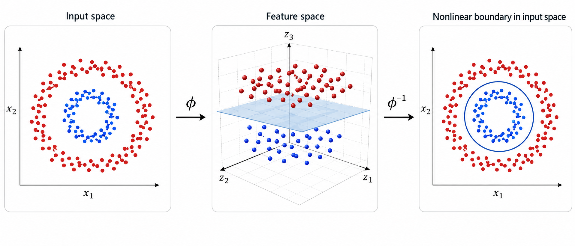
Recall now (with the help of the following figure from our discussion of SVCs) that data that are difficult to tackle in their original space may actually be much easier to deal with in a non-linearly transformed space:
13.4.3.2 Working with Kernels
Kernel PCA is the idea of applying PCA to a nonlinear transformation of the data, where every point $x^{(i)}$ is (implicitly) mapped via a transformation $\phi$ to a point $\phi(x^{(i)})$. The problem is that the transformation $\phi$ may not be given, and so we don't have the transformed points. Notice however that the Kernel-based PCA only requires access to the similarities between the points (that is, the inner products). So, rather than computing $$ K_{ij} = \phi(x^{(i)})^T \phi(x^{(j)}) \, , $$
we can simply compute it as $$ K_{ij} = \kappa(x^{(i)},x^{(j)}) $$
where $\kappa$ is some other appropriate kernel function.
Consider for example the Radial Basis Function kernel where we have $$ \kappa(x,y) = exp(- \gamma(\|x - y\|^2) \, , $$
which takes the Euclidean usual distance and converts it to a similarity value using an exponential decay function, where $\gamma$ is a parameter. Note that when $x=y$, this is equal to $1$, which also happens with the cosine similarity (assuming the norm of the vector is 1). On the other hand, when $x$ and $y$ are less aligned, then $\kappa(x,y)$ tends to 0.
There is a very nice theory about what functions can become kernels, and usually we pick this based on an intuition about what constitutes a good similarity between data points. There are some standard kernels that one can use, such as the polynomial kernel $$ \kappa(x,y) = (x^T y + \theta)^p \, $$ where $\theta$ and $p$ are parameters.
Kernel PCA in this non-linearly transformed space can be performed by first computing the kernel matrix $K$, where we apply the kernel function to each pair of points in order to compute $K_{ij}$. The next step would be to compute the $k$ eigenvectors of the matrix $K$ — however a little more care is needed. When we compute the 'linear' kernel $K = XX^T$, the matrix $K$ already has columns and rows that sum to zero. Data centered in this way tends to be more numerically stable than data that does not have this property.
Nonlinear kernel matrices are typically not centered, and so in practice we need to apply a straightforward centering operation. So, with our centered $K$, we can now find the top $k$ eigenvectors. These will be now of dimension $n$, and will actually be the projections of our non-linearly transformed points to the principal components of their covariance matrix.