Module 14 — Unsupervised Clustering
So far in this course we have studied strategies for supervised learning, which rely on training data to develop a model from which predictions can be made. Sometimes, however, we would like to explore a data set for which we know little, and for which training data may not be available. In such cases, unsupervised learning techniques could be useful in gaining an initial understanding of the nature of the data.
In this module, we will discuss a form of unsupervised learning called clustering, in which the goal is to form groups within the input dataset (the 'clusters'), such that:
- Points within each group are well associated according to some measure of similarity.
- Points drawn from different groups are well differentiated.
Clustering has been the topic of an enormous research effort over many decades, and a huge literature in this area exists. Here, we will look at a few of the most commonly-used clustering methods.
14.1 k-Means ⬤ 
Distance-based clustering methods usually require that some notion of similarity (or distance) be defined for the data, and an objective function be provided. In its standard form, the famous $k$-means algorithm assumes that
- the datapoints are represented as points in a $d$-dimensional space, and
- the clustering is defined by $k$ choices of representative locations in the space.
14.1.1 Problem Statement
Given a dataset $X\subset\mathcal{R}^d$, partition $X$ into $k$ disjoint clusters $X^{(1)}, \ldots, X^{(k)}$ such that, if $\mu_1,\ldots,\mu_j$ is the average of the points of cluster $X^{(j)}$, the following quantity is minimized:
$$ \mathit{distortion} = \sum_{j=1}^k \sum_{x \in X^{(j)}} \|x-\mu_j\|_2^2 \, .$$
These averages (also called the cluster 'means', 'representatives', 'centers', or 'centroids'), are obtained by summing all the point vectors assigned to the cluster, and dividing by the number of points:
$$ \mu_j \: = \: \frac{1}{|X^{(j)}|} \sum_{x\in X^{(j)}} x \, .$$
The cluster representatives can be viewed as approximations of its cluster members, from which the distance of each member is a form of 'error' or 'distortion' or 'loss'. Minimization of the $k$-means distortion formula is equivalent to the minimization of the mean squared error (MSE) from a prediction of location as given by the cluster representative.
14.1.2 Standard k-Means Algorithm
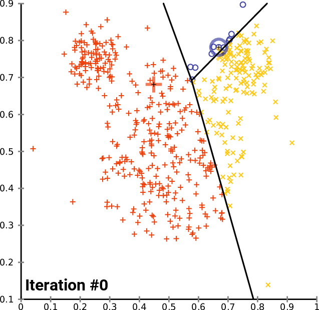
The $k$-means algorithm is an iterative process, in which two steps are alternated — the assignment step and the update step — until some converge criterion is reached.
- Random initialization: Choose $k$ data points at random as the initial cluster centers $\mu_1, \ldots, \mu_k$.
- Assignment step: Assign each point to its nearest center $\mu_j$. This produces a set of cluster members $X^{(j)}$ with $\mu_j$ as their representative.
- Update step: Calculate a new representative for cluster $j$ using the update formula $$ \mu_j \: \leftarrow \: \frac{1}{|X^{(j)}|} \sum_{x\in X^{(j)}} x \, .$$
- Repeat Steps 1 and 2 until convergence.
From Wikipedia (https://en.wikipedia.org/wiki/File:K-means_convergence.gif)
The standard algorithm has a number of advantages and disadvantages.
Advantages:
- The algorithm is very simple to implement!
- When $k$ is small compared to $n$, each iteration is very fast. The time required is proportional to $ndk$.
- Usually, not many iterations are required (but see the comment on convergence below!).
- The partition of space produced is a proximity map (a so-called 'Voronoi diagram'), which is known to have interesting mathematical properties.
Disadvantages:
- The distortion objective function favors the production of spherical clusters.
- The algorithm is not guaranteed to find a minimum-distortion clustering — it can get stuck at a local minimum.
- The performance is very sensitive to the initial choice of cluster centers.
- Convergence can be very slow. In practice, a stopping criterion is needed.
14.1.3 Variant Algorithm: k-Means++
In the animation of $k$-means shown above, the random initialization step produced two cluster centers very close to one another. When the initial set of centroids are not well spread out among the data, convergence may take longer, and the quality of the final clustering may suffer as a result.
To counter this, many different initialization strategies have been proposed. The popular $k$-means++ algorithm addresses the problem of initialization by encouraging the cluster centers to have greater separation within the dataset.
This is done by first choosing one point (uniformly) at random to be a cluster center, and then iteratively selecting the next centers with probability determined according to the following rule:
- Let $M$ be the set of cluster centers selected thus far.
- Let $\mathit{dist}_i$ be the distance from an unselected data point $X_i$ to the nearest cluster center in $M$.
- Generate a probability $p_i$ for the selection of $X_i$ as the next cluster center: $$ p_i = \mathit{dist}_i \bigg/ \sum_{x_t\in X\setminus M} \mathit{dist}_t \, . $$
The probability $p_i$ can be simply stated as the distance from $X_i$ to its closest cluster center, taken as a proportion of the total such distances for all points eligible to be selected. When $X_i$ is located close to one of the cluster centers, its chance of selection is therefore small. When it is far from any cluster center, its probability is then relatively large.
Overall, this simple and elegant strategy encourages dispersion of the cluster centers while still preserving the advantages of a random selection.
14.2 Agglomerative Hierarchical Clustering ⬤ 
Another way of producing a clustering is through agglomeration — that is, by building up larger clusters through successive merging of smaller clusters. To do this, we need a policy by which we can decide which clusters should be merged at any given step. The way this is managed is through some notion of a distance between clusters.

14.2.1 Linkage Policies
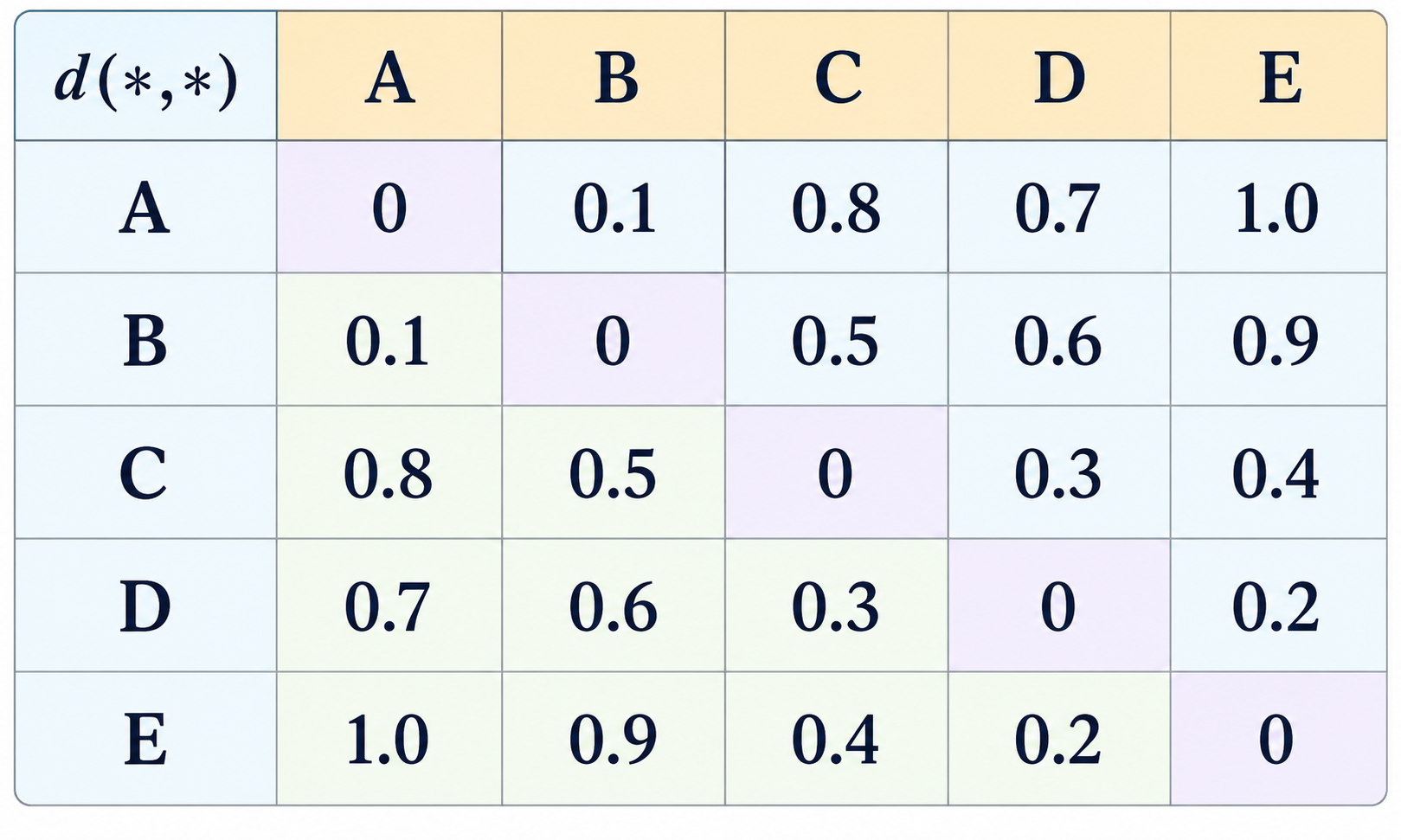
At each step of agglomerative clustering, two clusters are merged. Of all the candidate pairs, the one with smallest inter-cluster distance is chosen.
There are several common ways in which the distance between two clusters $A$ and $B$ can be defined. These include:
- Single linkage: (Also called Nearest Neighbor.) The distance between $A$ and $B$ is determined by the closest pair of cluster members $(a,b)$ such that $a$ is $A$, and $b$ is in $B$. $$ d_{\mathit{single}}(A,B) \: = \: \min_{a\in A; b\in B} \mathit{dist}(a,b) \, . $$
- Complete linkage: (Also called Farthest Neighbor.) The distance between $A$ and $B$ is determined by the farthest pair of cluster members $(a,b)$ such that $a$ is $A$, and $b$ is in $B$. $$ d_{\mathit{complete}}(A,B) \: = \: \max_{a\in A; b\in B} \mathit{dist}(a,b) \, . $$
- Average linkage: The distance between $A$ and $B$ is the average of the distances between pairs of cluster members $(a,b)$ such that $a$ is $A$, and $b$ is in $B$. $$ d_{\mathit{average}}(A,B) \: = \: \frac{1}{|A|\cdot|B|}\sum_{a\in A}\sum_{b\in B} \mathit{dist}(a,b) \, . $$
- Mean linkage: The distance between $A$ and $B$ is the distance between their cluster centers. $$ d_{\mathit{mean}}(A,B) \: = \: \mathit{dist}(\mu_A, \mu_B) $$ where $$ \mu_A \: = \: \frac{1}{|A|}\sum_{a\in A} a \:\:\: \mathrm{and} \:\:\: \mu_B \: = \: \frac{1}{|B|}\sum_{b\in B} b \, . $$
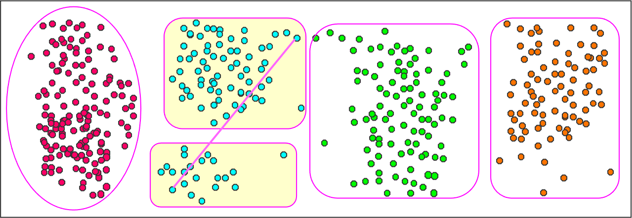
Before merging:
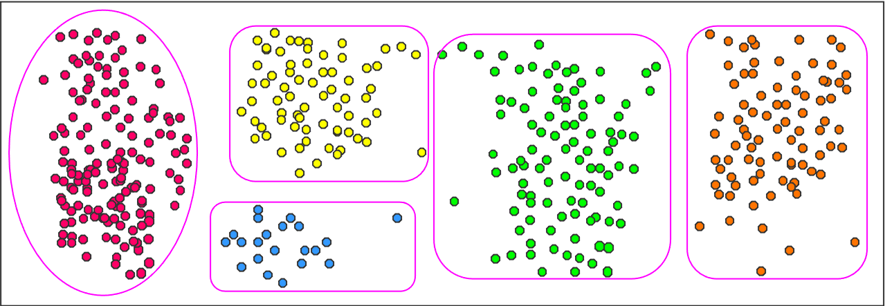
After single-linkage merge:
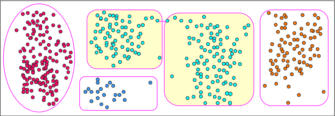
After complete-linkage merge:
14.2.2 Agglomerative Clustering
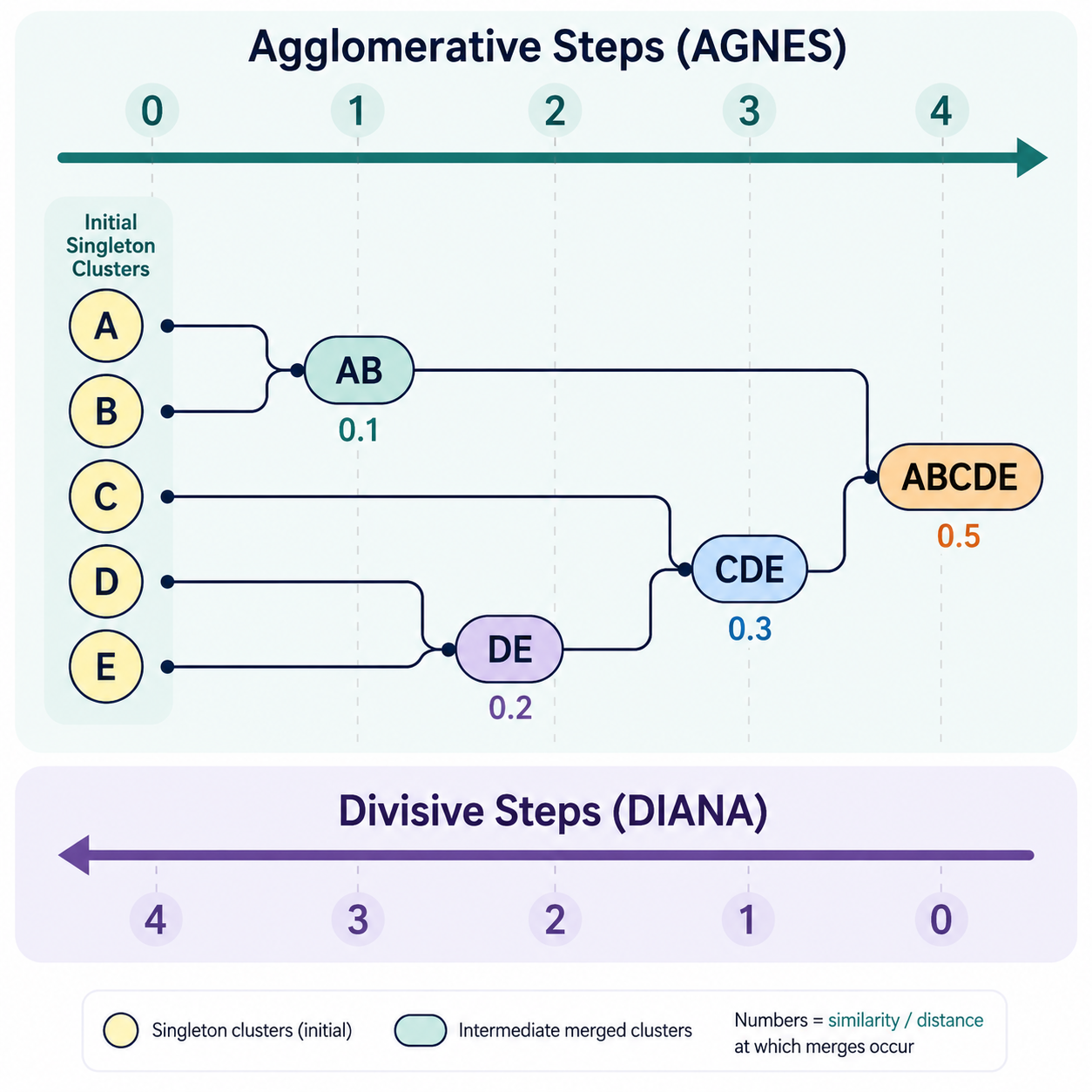
The basic form of agglomerative clustering, AGNES (AGlomerative NESting), dates back to the work of Kaufman and Rousseeuw in 1990. In AGNES,
- Every datapoint is initially in its own cluster.
- The two closest clusters are merged.
- Inter-cluster distances are updated.
- Steps 1 and 2 are repeated until a desired number of clusters $k$ is reached.
At each step, the number of clusters is reduced by 1 with each merge, until the target number is reached. Along the way, a history of the merges can be produced in the form of a collection of trees, whereby:
- A node is created for each cluster produced.
- Whenever two cluster nodes are merged, they are each linked to the new cluster node.
Often, the algorithm is run until all points are members of a single cluster. In this case, the history consists of a single merge tree (called a dendrogram) that can be analyzed to determine an appropriate number of clusters $k$.

During the execution of the algorithm, the merge distance never decreases, since the smallest available inter-cluster distance is always chosen. This fact can be used by an algorithm to organize the data for more efficient merge handling and updating.
Agglomerative clustering is computationally expensive. As originally designed, AGNES requires time proportional to $n^3$, where $n$ is the number of data points. Since then, more efficient implementations have been developed (particularly for single-linkage clustering), but none can do better than $O(n^2)$.
Kaufman and Rousseeuw proposed another variant of hierarchical clustering along with AGNES, in which a top-down 'divisive' approach is taken instead of bottom up. Their original method, DIANA (DIvisive ANAlysis) runs like AGNES but in reverse, with cluster splits instead of merges.
- All datapoints are initially in a single cluster.
- Among all current clusters, one is chosen for splitting. The split is the one that produces the greatest possible inter-cluster distance between the two new (smaller) clusters.
- Inter-cluster distances are updated.
- Steps 1 and 2 are repeated until a desired number of clusters $k$ is reached.
If run until every point is in its own cluster ($k=n$), DIANA produces the same dendogram as AGNES. Due to the complexity of determining the best split, faster heuristics (such as $k$-means!) are often used.
14.2.3 The Effect of Linkage Policies
In agglomerative (or divisive) hierarchical clustering, the various linkage policies have a great effect on the quality and nature of the clusterings produced.
Here are some of the characteristics of each.
Single linkage: Although single-linkage is the only policy known to be able to produce an optimum solution in $O(n^2)$ time, it suffers from an effect called chaining. As the name suggests, the strategy can lead to incoherent clusters consisting of long chains of points, where the members at each end have little or no similarity to each other.
Complete linkage: By seeking to minimize the distance between the farthest pair of data points, the complete linkage merge policy favors the formation of compact, rounded clusters — the opposite effect of chaining. However, the merge order is highly influenced by outliers.
Average linkage: This method has the advantage of being less affected by outliers than complete linkage, while avoiding the tendency to form chains. However, the cost of average linkage is very high, since a quadratic number of distances are computed.
Mean linkage: This method has advantages similar to those of average linkage. Moreover, mean linkage is very efficient, since the computation of the two cluster means is linear in the size of the clusters. However, like $k$-means, this linkage policy requires that the data points can be averaged (for example, real-valued as opposed to categorical).
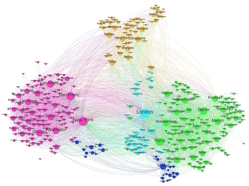
Social network graph (2011), from Wikipedia (https://commons.wikimedia.org/wiki/File:The_true_continents_of_the_world_(version_2)_(5923004341).jpg)
_(5923004341).jpg)
14.3 Graph-based Clustering ⬤ 
Let's now consider a different kind of clustering, where the input data is not represented by points in space, but instead as the nodes and edges of a graph or network. Here, the clustering task is to partition the nodes into $k$ groups for which:
- The nodes of each group have many interconnections (edges) among them.
- There are relatively few interconnections between different groups.
An example of graph data for which clustering is an interesting problem is that of social networks such as the one depicted above, where nodes represent people or locations, and edges represent significant traffic or communication between them.
14.3.1. Spectral Graph Clustering
Here, we will assume that we are given an undirected graph; that is, one in which the edge between two nodes indicates a mutual relationship between the two.
An undirected (simple) graph can be represented by an adjacency matrix $A$, where
- a value of $A_{ij} = 1$ indicates that an edge exists between node $i$ and node $j$, and
- a value of $A_{ij} = 0$ indicates that no such edge exists.
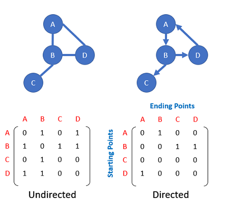
To this, we introduce the notion of a diagonal matrix $D$, in which:
- Every entry $D_{ii}$ on the diagonal is equal to the degree of node $i$ — that is, it equals the number of edges in which the node participates.
- All entries of $D$ not on the diagonal are equal to 0.
Next, we consider the matrix $M$ defined as $M=D^{-1}A$. Matrix $M$ can be thought of as a probability-weighted adjacency graph. Imagine that each node is to choose one of its adjacent edges at random. The entries of $M$ indicate the probability of a given edge being chosen in this way.
For the above example, the matrix $D$ is $$ D = \left( \begin{array}{cccc} 2 & 0 & 0 & 0 \\ 0 & 3 & 0 & 0 \\ 0 & 0 & 1 & 0 \\ 0 & 0 & 0 & 2 \\ \end{array} \right) \, , $$ and $M$ is $$ M = D^{-1}A = \left( \begin{array}{cccc} 1/2 & 0 & 0 & 0 \\ 0 & 1/3 & 0 & 0 \\ 0 & 0 & 1 & 0 \\ 0 & 0 & 0 & 1/2 \\ \end{array} \right) \left( \begin{array}{cccc} 0 & 1 & 0 & 1 \\ 1 & 0 & 1 & 1 \\ 0 & 1 & 0 & 0 \\ 1 & 1 & 0 & 0 \\ \end{array} \right) = \left( \begin{array}{cccc} 0 & 1/2 & 0 & 1/2 \\ 1/3 & 0 & 1/3 & 1/3 \\ 0 & 1 & 0 & 0 \\ 1/2 & 1/2 & 0 & 0 \\ \end{array} \right) \, . $$
To find a clustering of the graph, we compute the first $k$ eigenvectors of $M$, and concatenate them as the columns of a new $n\times k$ matrix $Y$.
What we have done here is a form of dimensionality reduction, where we have replaced the original $n\times n$ adjacency matrix $A$ by an $n\times k$ matrix $Y$, which can then be treated as $n$ data points (one for each node), located in a $k$-dimensional real-valued space.
Now, the data is in a form where we can use any of our favorite algorithms for clustering real-valued data! A typical choice for this is $k$-means++. Once we have the clustering, the groups formed can be read directly as the clusters of nodes.
Why this works well is a matter of a deep and rich mathematical theory with connections to the study of random walks in networks (among many other things). The eigenvalues of the adjacency graph are called its spectrum, which is where the term 'spectral graph clustering' comes from.
14.3.2 Spectral Clustering
Next, we will see how spectral graph clustering can be used to help us with difficult clustering problems involving our familiar representations of data as points in space.
For data in which the natural groupings are non-convex and highly interwoven, many (if not most) of the standard clustering techniques fail spectacularly. Consider the dataset in the left-hand image below. We as humans can easily judge it to be composed of two natural clusters in the form of interwoven spirals. However, applying a representative-based clustering method such as $k$-means would be disastrous, cutting through these clusters as in the middle image.
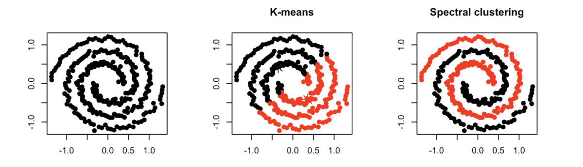
One way of dealing with such cases is to impose a graph structure on the data, by connecting each point to its $K$ nearest neighbors. In doing so, we use this graph as a way of discovering the shape of the data. Once we have the graph, we can then use spectral graph clustering to extract these shapes, as shown in the right-hand image. We usually call this method spectral clustering instead of 'spectral graph clustering', to emphasize the fact that the input is unstructured point data instead of a graph.
Spectral clustering is somewhat related to single-linkage hierarchical clustering, in that simple neighborhood information can be used to find long chains as clusters. However, with a good choice of $K$ (usually small), spectral clustering can be far more robust. This is because the local connections for choices of $K>1$ are denser than can be achieved using single linkage clustering.