Module 15 — Introduction to Artificial Neural Networks
15.1 Connecting Neurons Together: 2-Layer Networks ⬤ 
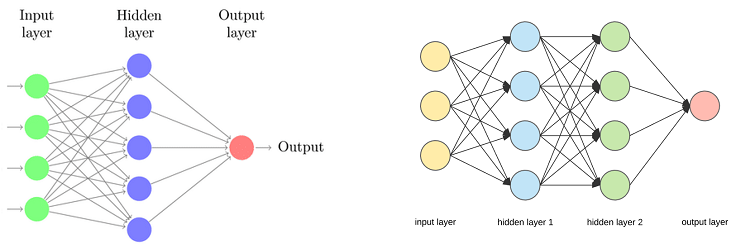
So far we have discussed single neurons, including the logistic neuron that takes as input a vector $x$, modulates it by a weight parameter vector $w$, computes the net input $z$, and finally outputs the activation function, e.g. $\sigma(z)$.
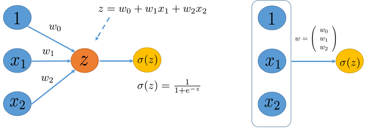
The figure on the left shows a single neuron, and the figure on the right is a more concise version of it.
We have also seen the One-vs-Rest method, which can be regarded as combining the predictions of multiple outputs coming from different neurons, as shown in the figure below.
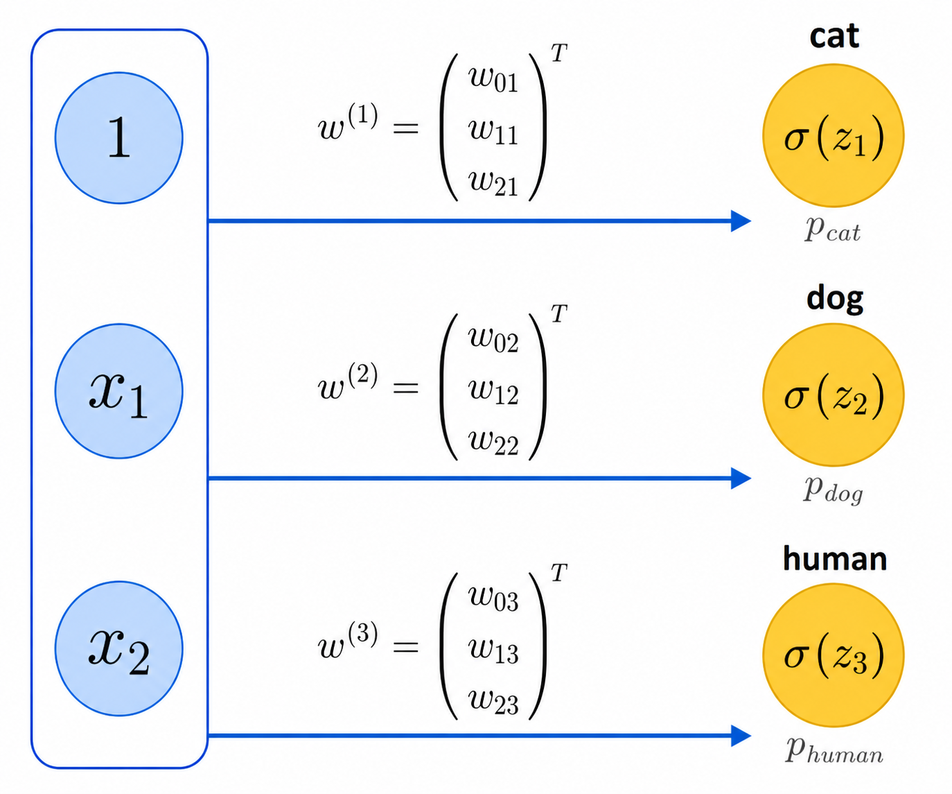
Each of these output neurons can be trained independently (in parallel with the others), and so we can view them as an entire output layer. The combined input-output layers together form a primitive 2-layer neural network. We should not forget that this type of network is still able to separate the space only with hyperplanes.
15.2 Connecting Neurons Together: 3-Layer Networks ⬤ 
Neural networks become much more interesting when we add one intermediate (also called hidden) layer of neurons as shown in this picture:
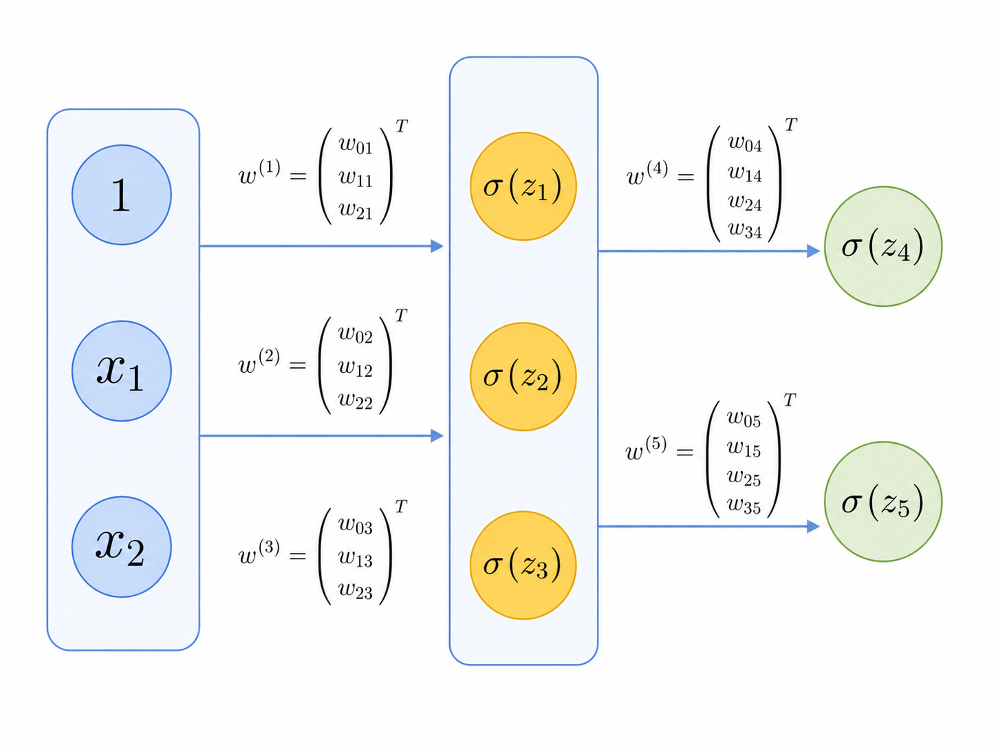
This is still a simple 'device' that has a forward mode that takes one input $x$ and computes an output. The simple but important difference is that the neuron in the output layer takes as its inputs the activation values of the hidden layer. More specifically, if $\sigma(z_1), \sigma(z_2), \sigma(z_3)$ are the outputs of the hidden layer neurons, then the output of Neuron 4 (in the output layer) will be:
$$ \sigma(z_4)\,, \:\:\:\mathrm{where}\:\:\: z_4 = w_{04} + w_{14}\sigma(z_1) + w_{24}\sigma(z_2) + w_{34}\sigma(z_3) \, . $$
In other words, after the outputs of the hidden layer are computed and become available, then each neuron in the output layer can use them to calculate the final output. We should note here that each neuron in the network has its own dedicated set of weights, exactly the way it would happen in a brain: each neuron has its own dedicated set of dendrites.
15.3 Training 3-Layer Networks ⬤ 
A 3-layer neural network is still a simple device that takes an input $x$ and computes an output. For example, the neural network in the above picture will compute two outputs $[\hat{y}_4,\hat{y}_5]$ that we can then compare with the true labels $[{y}_4,{y}_5]$ and calculate a loss for the point $x$. We can then aggregate all individual losses, which gives rise to a loss function $L(X,y,W)$ that depends on the data and on all weights $W$. Our goal will be to learn the weights $W$ that minimize the loss, and we can do that by using one of the optimizers we have learned about. So, everything we have learned for simple single-neuron models applies in nearly the same way for neural networks.
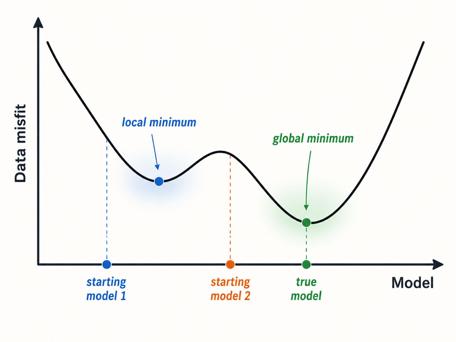
However, one important difference is that unlike the single-neuron models where loss functions are convex and mathematically well-understood, the 'loss landscape' for 3-neural networks is much more complex, with many local minima, as illustrated in the picture below. Such local minima make training a more challenging task. But while gradient descent-based optimizers will become stuck at local minima most (or nearly all!) of the time, neural networks are still able to generalize better than simple neurons. Developing a theoretical understanding of the generalization performance of neural networks is a significant open problem in Machine Learning.
15.4 Universal Approximation Theorems — and More Layers ⬤ 
We have seen that 2-layer neural networks (NNs) can only represent linear surfaces and functions. Surprisingly, adding that one hidden layer in 3-layer NNs increases their power formidably.
There are various mathematical theorems known as universal approximation (UATs) theorems [1] that very roughly state the following:
- If the training dataset $(X,y)$ comes from a 'reasonable' function $y=f(X)$ (where reasonable means almost any function you can imagine), then there exists a 3-layer neural network $m$, such that $m(X)$ approximates $f(X)$ arbitrarily well, i.e. the loss function of $m$ can be driven to be very small on $X$.
UATs imply that 3-layer networks can represent/learn any reasonable function and, in that sense, adding a second hidden layer does not increase the fundamental power of neural networks. However, UATs merely state the existence of a good 3-layer network, but such a network may be too big (i.e. with a very large hidden layer), or it may be very difficult or even impossible to train in order to discover the appropriate setting for its parameters, so that it approximates the desired function $f$.
While adding more hidden layers does not increase the representation power of neural networks, it has the potential to reduce the number of required parameters for learning the function $f$, change the landscape of the loss function, and result in better generalization. For that reason, much of the current research in Machine Learning and Deep Learning revolves around discovering better architectures, with different numbers and types of hidden layers. In other words, the entire architecture of a NN becomes itself a key hyperparameter, and gives a vast number of possible machine learning algorithms and models for any given learning problem.
15.4.1 Universal Approximation Theorems — and the Risk of Overfitting
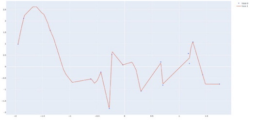
In practice, UATs also imply that neural networks have a capacity for overfitting to the training data. Consider for example the outcome of training a 3-layer network for regression, with a random training set as input. The neural network is able to almost match the training points — that is, its loss value is very small. In some sense, the network is able to 'learn' a pattern, when no such pattern exists, which of course means overfitting.
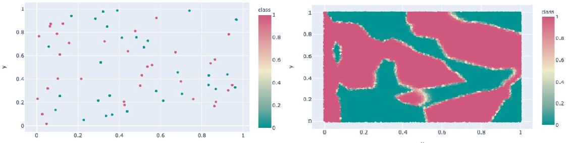
Another example is shown in the picture below: a random set of 2D points with random labels can still be separated by a 3-layer network.
15.5 Algebra of Forward Calculation ⬤ 
As we described in section 15.1, it is not very difficult to do the forward calculation one neuron at a time. However, it is useful to think about the entire calculation in terms of matrices.

Consider as an example the above neural network. Each of these three neurons has its own dedicated set of weights, and we can make them columns of a matrix of weight parameters, as follows:
$$ W_{\mathrm{ih}} = \left( \begin{array}{ccc} w_{11} & w_{12} & w_{13} \\ w_{21} & w_{22} & w_{23} \\ \end{array} \right) \, . $$
Then, for a given input $x_{\mathrm{in}} = [x_1, x_2]$, the three net inputs $z_1,z_2,z_3$ will be the three entries of the row vector
$$ z_{\mathrm{h}} = x_{\mathrm{in}}\cdot W_{\mathrm{ih}} + [w_{01}, w_{02}, w_{03}] \, . $$
After computing $z_{\mathrm{h}}$ we can in one step calculate the signmoid of its entries, which will give us the activations $a_{\mathrm{h}}$ for the three neurons.
Similarly, we can define another matrix $W_{\mathrm{ho}}$ that contains the weights between the hidden and the output layer. Then, the forward calculation of the entire network will be
\begin{array}{ccl} z_{\mathrm{h}} & = & x_{\mathrm{in}}\cdot W_{\mathrm{ih}} + [w_{01}, w_{02}, w_{03}] \, , \\ a_{\mathrm{h}} & = & \sigma(z_{\mathrm{h}}) \, , \\ z_{\mathrm{o}} & = & a_{\mathrm{h}} \cdot W_{\mathrm{ho}} + [w_{04}, w_{05}] \, , \\ a_{\mathrm{o}} & = &\sigma(z_{\mathrm{o}}) \, . \end{array}
Keep in mind that we can make the representation even more compact by augmenting the input vector $x_{\mathrm{in}}$ to be $[1, x_1, x_2]$, and the weight parameter matrix $W_{\mathrm{ih}}$ to be $$ W_{\mathrm{ih}} = \left( \begin{array}{ccc} w_{01} & w_{02} & w_{03} \\ w_{11} & w_{12} & w_{13} \\ w_{21} & w_{22} & w_{23} \\ \end{array} \right) \, . $$ With this form of augmentation, the forward calculations can be very simply expressed; for example, \begin{array}{ccl} z_{\mathrm{h}} & = & x_{\mathrm{in}}\cdot W_{\mathrm{ih}} \, . \end{array}
15.5.1 Forward Calculation with a Batch
When $x_{in}$ is a single point, then $a_h$ and $a_o$ are also vectors of dimension equal to the number of units in the corresponding layer.
However, we often want to evaluate multiple points together, for example when we do batch gradient descent. In that case we will have as input a batch $X_{in}$ of dimensions $s\times d$, where $s$ is the size of the batch, and $d$ is the number of input features. The math of the forward calculation is precisely the same:
\begin{array}{ccl} z_{\mathrm{h}} & = & X_{\mathrm{in}}\cdot W_{\mathrm{ih}} + [w_{01}, w_{02}, w_{03}] \, , \\ a_{\mathrm{h}} & = & \sigma(z_{\mathrm{h}}) \, , \\ z_{\mathrm{o}} & = & a_{\mathrm{h}} \cdot W_{\mathrm{ho}} + [w_{04}, w_{05}] \, , \\ a_{\mathrm{o}} & = &\sigma(z_{\mathrm{o}}) \, . \end{array}
In this case though, $a_{\mathrm{h}}$ and $a_{\mathrm{o}}$ are also batches, i.e. 2D matrices with $s$ rows. In particular the $i$-th row of $a_{\mathrm{h}}$ or $a_{\mathrm{o}}$ corresponds to the point in the $i$-th row of $X_{\mathrm{in}}$.
15.6 Notebook Illustrating the Forward Operator ⬤ 
Here is the code notebook.
15.7 Backpropagation for Training ⬤ 
Neural networks are trained using the same approach we used for single neurons. We define a loss function, we calculate it, and then we use gradients to go closer to a local minimum. The main challenge is that the partial derivatives of the loss function with respect to the weights have more complicated dependencies. However, we can actually compute these derivatives, by following a process known as backpropagation.
We will illustrate the process by training a single sigmoid neuron.
Let's first recall how we learn the parameters in the logistic regression. The general approach is as follows:
Define a cost function $C(w)$, which only depends on the set of weights
Calculate the derivative of $C(w)$ with respect to every weight $w_i$, which is denoted as $$\frac{\partial C(w)}{\partial w_i}.$$
Update every weight as follows:
$$ w_i:= w_i - \eta \frac{\partial C(w)}{\partial w_i}. $$
Here $\eta$ is the learning rate.
We saw that the cost depends on all points so the gradient descent algorithm needs to read all points in order to calculate the derivatives. We also said that in order to avoid that (and converge faster) we can work with mini-batches, or even single points.
We have previously done a derivation of the gradient descent rule for the linear regression model. We only showed the rule for the logistic regression, which was derived by maximizing the likelihood measure.
In order to see the essense of backpropagation we will try to see how it works in the single neuron case. Take a look at the following picture:
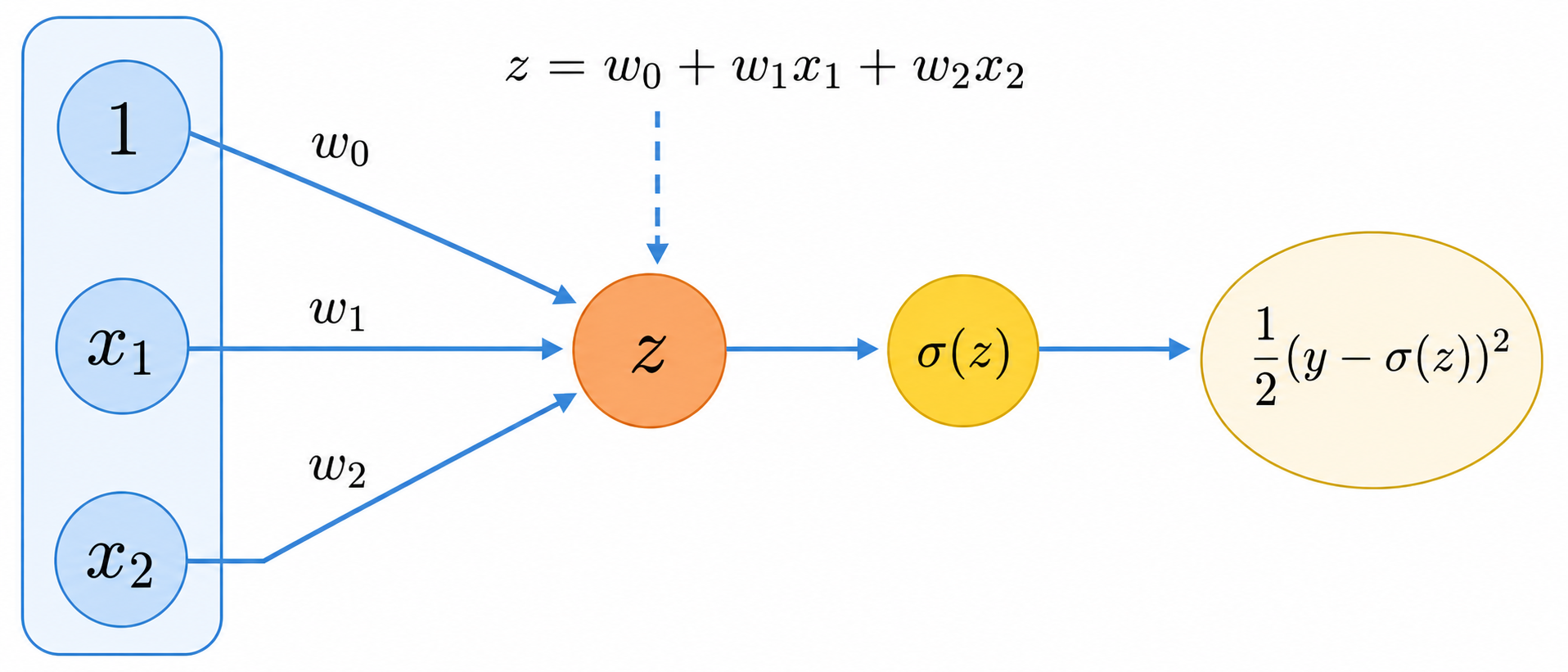
This looks exactly like a single signoid neuron, but we just added one node to account for the error contributed by one point. This point will also contribute a summand to the gradient.
So, here we have $$ \mathit{loss} = \frac{1}{2} (y - \sigma(z))^2 \, , $$ but we want to compute the derivative, with respect to (say) $w_1$.
So, we can ask the following sequence of questions:
- What is the 'rate of change' of the error with respect to $\sigma(z)$? That means we take the derivative where we treat $\sigma(z)$ as one variable and we have:
$$ \frac{\partial\, \mathit{loss}}{\partial \sigma(z)} = - (y - \sigma(z)) $$
- What is the 'rate of change' of $\sigma(z)$ with respect to the net input $z$? That means we take the derivative of the sigmoid with respect to $z$, and we have:
$$ \frac{\partial\, \sigma(z)}{\partial z } = \frac{\partial\, (1+e^{-z})^{-1}}{\partial z } = -(1+e^{-z})^{-2} (-e^{-z}) = \frac{1}{1+e^{-z}} \cdot \frac{e^{-z}}{1+e^{-z}} = \sigma(z)(1-\sigma(z)) $$
- What is the 'rate of change' of $z$ with respect to the weight $x_1$? We have
$$ \frac{\partial z}{\partial w_1} = x_1 $$
So, since we have all these relative 'rates of change' we can actually calculate the speed of the error with respect to $w_1$. And this is given by multiplying all these relative speeds together (which is known as the 'chain rule' in calculus):
$$ \frac{\partial\, \mathit{loss}}{\partial w_1} = \frac{\partial\, \mathit{loss}}{\partial\,\sigma(z)} \cdot \frac{\partial\,\sigma(z)}{\partial z} \cdot \frac{ \partial z}{\partial w_1} = - (y - \sigma(z)) \sigma(z)(1-\sigma(z)) x_1 $$
This in other words would be the update we will do in $w_1$, due to the particular point $(x,y)$. This looks different from the update rule we have seen earlier, but this is only because we minimize a different type of error.
The important point here is this:
In order to find the derivative we were looking for, we kept asking questions and doing calculations in a 'backward' manner, starting from the output all the way to the parameter $w_1$. This is essentially what back-propagation does but in a more general way, going 'deeper' into the layers of a multi-layer network. The essence of this is that we compute quantities for the parameters of all units in a layer, and after doing that, we can 'push' these quantities to the prior layer and continue our computation there.
15.7.1 Deeper Backpropagation
To train a network with 3 or more layers, we will follow exactly the same approach: We will try to minimize an error function $E$, and we will do that by computing derivatives (gradient terms) of the error, by backpropagating questions and calculations. The exact calculations are somewhat tedious, but in fact they can be carried out even automatically (by automatic differentiation programs).
Let's look at a snapshot of a calculation for a weight going from the input to the inner layer.
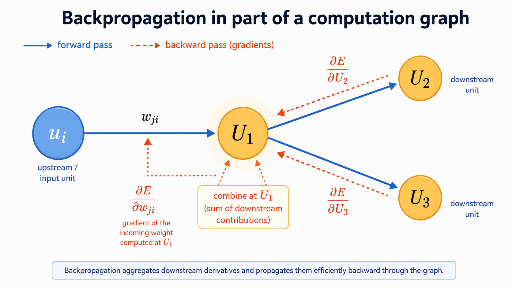
Here we see that in order to calculate $\partial E/ \partial w_{ji}$ we will first ask and calculate derivatives of the activations for the units $U_2$ and $U_3$, and then we will find derivatives $\partial E/ \partial U_2$ and $\partial E/ \partial U_3$ which will be then combined to find a derivative for $U_1$, and so on.
The bottom line is that these derivatives can all be calculated in parallel, via matrix operations. These are just provided as formulas in reference texts, and we will not be concerned them again, unless some of you would like to dig deeper into neural networks.
15.8 Hidden Layer as Learned Features ⬤ 
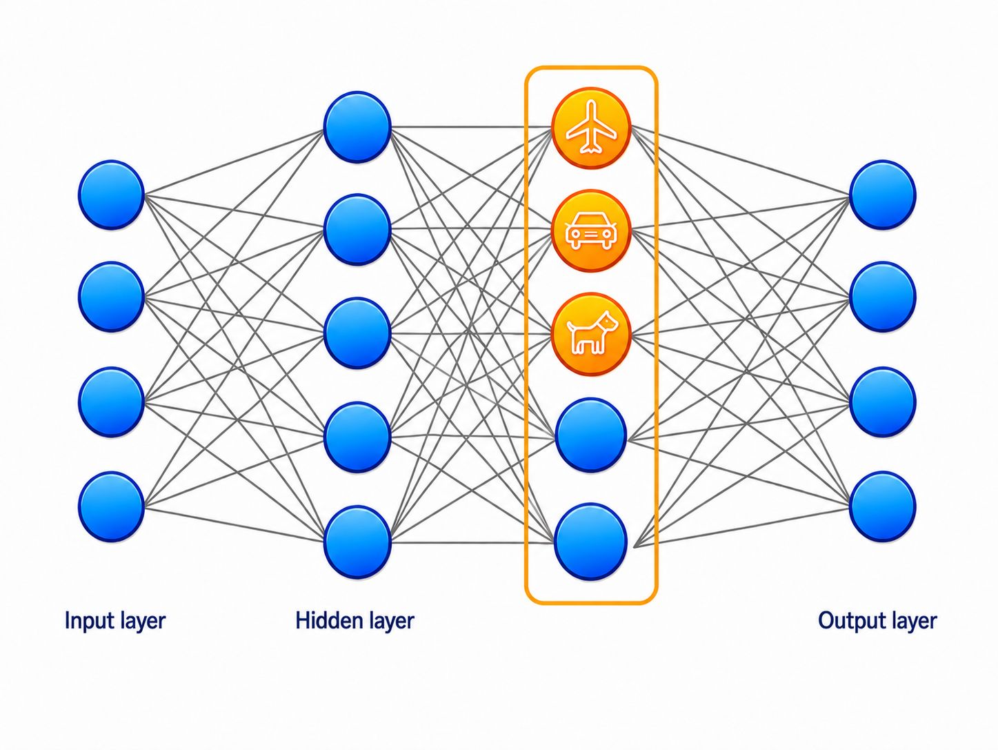
In previous chapters we have discussed the power of adding engineering features to our data. Of course, engineering appropriate features requires a deeper understanding of the data and its semantics, and further domain knowledge. Furthermore, the engineered features are fixed functions of the input data.