Module 16 — Nonlinear Layers, Softmax and Cross Entropy
16.1 Nonlinear Activations ⬤ 
Recall that so far we have discussed neural networks with layers of sigmoid neurons.
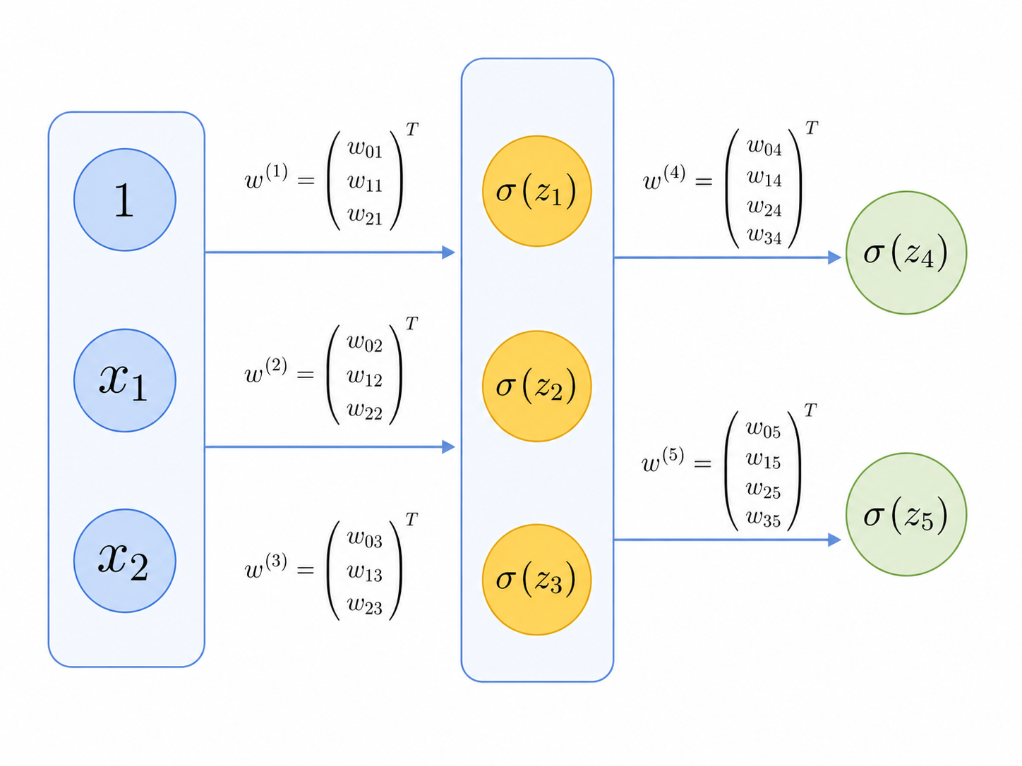
While having sigmoid functions in the output makes a lot of sense for classification problems, in principle there is no absolute necessity to use the sigmoid function in the neurons of the hidden layers. In general, hidden layer neurons can replace $\sigma(z)$ with some other nonlinear activation function $\phi(z)$. Some common choices include:
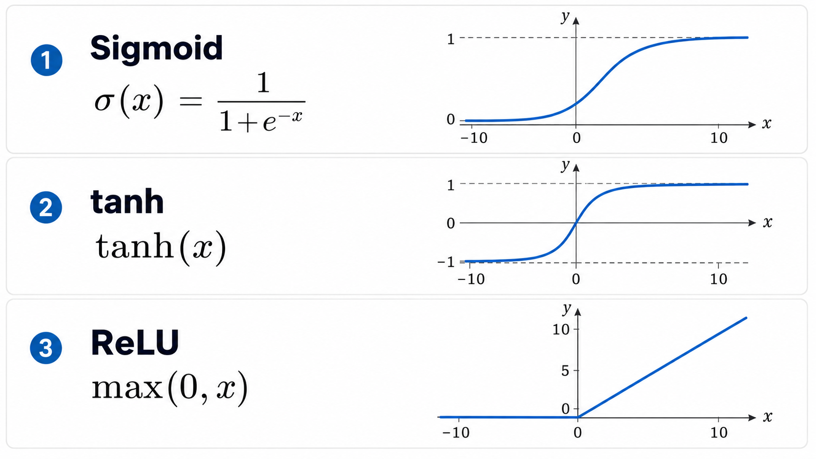
The hyperbolic tangent function $\phi(z) = tanh(z)$, which has 'step' behavior similar to that of the sigmoid function, but with a range between $-1$ and $1$.
The Rectified Linear Unit (ReLU), which is defined as $\phi(z)=z$ when $z\geq 0$ and $\phi(z)=0$ when $z<0$.
16.2 Softmax ⬤ 
In a classification problem with $k$ labels, one idea is to let the output layer consist of $k$ sigmoid neurons, where each neuron outputs a probability that the input is in the corresponding class. In this case, the sum of the $k$ outputs will not be equal to 1 — that is, it will not be a probability distribution.
The softmax layer adds one extra normalization calculation that ensures that the final output can be interpreted as a probability distribution. This is illustrated in the following picture:
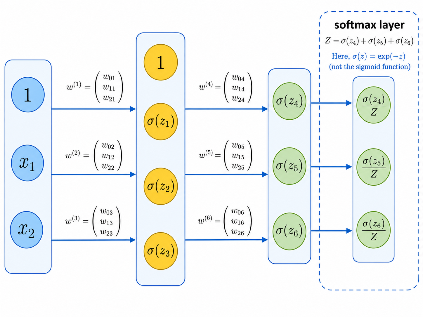
Please note, that in the softmax layer above we take $\sigma(z) = exp(-z)$.
16.3 Cross-Entropy Loss ⬤ 
The output/prediction of the softmax layer is a probability distribution $p = [p_1,\ldots,p_k]$ on the $k$ possible classes. The desired output can also be viewed as a probability distribution $q = [q_1,\ldots,q_k]$ which happens to be a bit more special: only one of the $q_i$'s is equal to $1$, and the rest are equal to 0. That is sometimes called a one-hot vector.
Then, since both the predicted and the desired output are probabilities, we can borrow notions from information theory to measure the 'distance' of these two probabilities, which could then be used as a type of loss for the given input point.
The cross entropy $\mathit{CE}(p,q)$ is defined as follows:
$$ \mathit{CE}(p,q) = - \left(\sum_{j=1}^k q_j \log_2 p_j \right) \, . $$
Note how this function is not symmetric with respect to $p$ and $q$. The reason we call it cross entropy is because $\mathit{CE}(p,p)$ is the standard entropy of the probability distribution $p$.
Recall that $p$ and $q$ are the predicted and desired output for a given point $X_i$. Denoting them by $p(X_i)$ and $q(X_i)$, respectively, we can use $\mathit{CE}(p(X_i),q(X_i))$ as a measure for the error on one point. For a batch of points $X$, the cross-entropy loss function is defined as:
$$ \mathit{CEL}(X) = \sum_{X_i \in X} \mathit{CE}(p(X_i),q(X_i)). $$
The cross-entropy loss function is the standard loss function implemented in common classifiers.
16.4 Notebook with MLP Classifiers in scikit-learn ⬤ 
Here is the code notebook.
Multilayer neural networks are called Multilayer Perceptrons in scikit-learn. It is worth taking a look at the scikit-learn documentation for MLP classifiers. A thing to notice is that all hidden layers must use the same type of neurons. The reason for that is that for each type of neuron, derivations for all the required backpropagation calculations have been hard-coded in the impementation. Newer tools such as PyTorch and TensorFlow have the capability to implement almost any arbitrary forward function.