Module 17 — Autoencoders
17.1 The Basic Idea ⬤ 
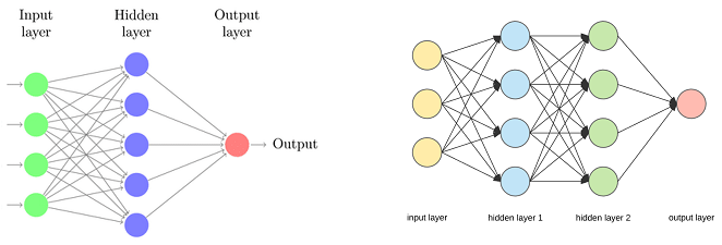
Neural networks were originally conceived as models for approximating functions $y=f(X)$. Most of the times the hidden layers of the neural networks are larger than the input layer, and the output layer size is determined by the type of supervised problem we want to solve.
Autoencoders are a very creative application of neural networks. The main ideas are these:
Standard neural networks are supervised models. Autoencoders are unsupervised models, where the desired output $Y$ is equal to the input $X$ (i.e. we have $Y=X$). That implies that the sizes of the input layers are equal.
The hidden layers are smaller than the input/output layers.
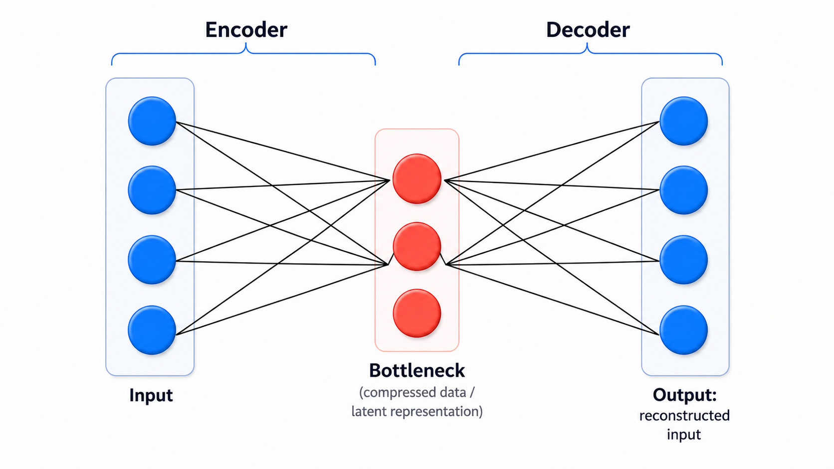
The following picture shows an autoencoder with one hidden layer.

Essentially the autoencoder's objective is to approximately reconstruct the input in the output layer, but do so by first 'compressing it' through the hidden layers.
The way this is done is via a loss function. More specifically, the network takes as input some point $X_i$ and returns an output $y_i = f(X_i,w)$ depending on $X_i$ and the weights of the network. We can then define a loss, such as the mean squared error:
$$ L = \sum_{i} (X_i - f(X_i,w))^2 \, . $$
We then use an optimizer to 'tune' the weights so as to minimize the loss function, which will happen if $X_i$ is approximately equal to the output of the network (in an average sense).
Of course, autoencoders can have multiple layers. A typical example is illustrated in this picture.
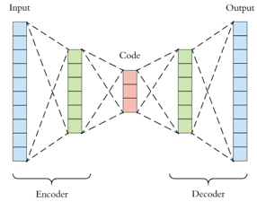
Typically, the hidden layers decrease in size up to the middle hidden layer, and then their sizes increase symmetrically up to the output layer. As usual the sizes of all layers are a hyperparameter of the architecture, and typically subject to experimentation.
17.2 Applications ⬤ 
If it is indeed possible to have a small value for the loss function, that really means that the data can be compressed down to the size of the hidden layer without losing too much information. In some sense, the autoencoder would learn the 'essential' part of the data. This intuition leads to a number of applications.
17.2.1 Dimensionality Reduction
Given an input point $x$, the activation values $a_h(x)$ of the bottleneck hidden layer can be viewed as learned lower-dimensional features. Because these features maintain the 'essential' information about the data, and because the autoencoder usually involves at least one layer that effects a nonlinear transformation, the autoencoder can be viewed as a nonlinear dimensionality reduction.
In fact, in a 3-layer autoencoder, disallowing all nonlinear activation functions at the hidden layer would produce a linear dimensionality reduction, that can be shown to be essentially equivalent to PCA! In other words, one can replace the entire sophisticated mathematical machinery of PCA with a simple neural autoencoder.
The following image shows the input and the output reconstructed image with a nonlinear autoencoder and with PCA (linear autoencoder) with target dimension equal to the hidden layer size.
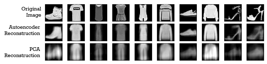
It can be seen that the reconstruction obtained via the nonlinear autoencoder is much better that the reconstruction obtained via PCA, which shows once again the power of nonlinearity.
Nonlinear dimensionality reduction can be used to get more efficient models (due to the smaller dimension), or it can also be used for implicit regularization — as 'smoothing out' the data details can sometimes improve generalization.
17.2.2 Denoising Autoencoders

Imagine we have a camera and we occasionally want to use it in conditions where there is noise (such as atmospheric disturbances, light artifacts, blurring, etc.). The input of the camera is $x+\epsilon$, where $x$ is the 'true' signal, and $\epsilon$ is noise that we would like to remove in order to recover the clear true signal $x$.
One way to do that is to start with a clean dataset $X$ (obtained when there is no noise in the environment) and for each point $X_i$, create a set $Z^{(\epsilon)}$ of noise data points $X_i + \epsilon_1, \ldots, X_i + \epsilon_j$, where $\epsilon_k$ are amounts of artificial or simulated noise.
We can slightly modify the autoencoder architecture and give as input the pairs $(Z^{(\epsilon)}, Z)$, where each $Z^{(\epsilon)}_i$ is a noise data point, and $Z_i$ is the corresponding original data point from $X$. Then, the loss function becomes:
$$ L = \sum_{i} (Z_i - f(Z^{(\epsilon)}_i,w))^2 \, . $$
If we are able to learn $w$ so that $L$ becomes small, we can effectively get rid of the noise. Thus the learned autoencoder-based architecture can work as device that denoises the data.
17.2.3 Outlier Detection
Suppose $f$ is an autoencoder trained on a dataset $X$. We can then compute for each point $X_i$ the individual reconstruction $\tilde{X}_i = f(X_i)$, and the reconstruction error $e_i = |\tilde{X}_i - X_i|$. Points with large reconstruction error must not have been effectively compressed in the bottleneck layer, and therefore a plausible explanation is that they are outliers in $X$. We thus have the potential of detecting outliers in $X$ by inspecting the reconstruction error.
17.2.4 Other Applications
There are many other applications of autoencoders; in particular, they are the basis of successful deep learning models for natural language processing. Autoencoders were originally proposed by Geoffrey Hinton [1], one of the key contributors in the recent deep learning wave.
17.3 Experiments with Autoencoders ⬤ 
Here is a code notebook on autoencoders.
In the first part, the notebook constructs an autoencoder for compressing 8 one-hot vectors into 3-dimensional representations, essentially learning the binary representations of the first 8 numbers.
In the second part, we train an autoencoder on a small dataset, and then apply k-means clustering on the original dataset, on the dimensionality-reduced dataset, and on the denoised/reconstructed input set.