Module 19 — Convolutional Neural Networks
19.1 Images as Feature Arrays ⬤ 
We begin with a refresher of how images are represented in a computer. A grayscale image is an array of features known as pixels, where each pixel is an integer in the range $[0,255]$ corresponding to the brightness of that spot in the image.

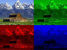
A color image consists of monochrome images on three different channels of feature arrays, corresponding to the red, green and blue colors. What we see in our displays is essentially the superposition of these three images.
19.2 Neural Networks for Images ⬤ 
So far we have worked with classification of grayscale images. The way we did it was to convert them into vectors (flatten them), by following a specified row-wise order for the pixels, and then feed them into a standard MLP classifier.
With the given row-wise order of the pixels, we learned a classifier $C_{\mathit{good}}$ that reaches 94% test accuracy.
It is interesting then to ask what would happen if we flattened the images according to some other random order for the pixels, where the same reordering is applied to all images. Then, instead of the original data matrix $X$ (of dimensions $n\times 784$), we would now have a data matrix $\hat{X}$ where the columns of $X$ have been shuffled.
Would there still be a good classifier for these rearranged vectors?
The answer is yes. The only thing we need is an appropriate reordering of the inputs of the classifier $C_{\mathit{good}}$. That would give us a new classifier $\hat{C}_{\mathit{good}}$ whose performance on $\hat{X}$ would be identical to the performance of $C_{\mathit{good}}$ on $X$. And, since we learned $C_{\mathit{good}}$ from a random initialization, it can be verified that with a random initialization we will also learn a similarly good classifier on the reordered training set.
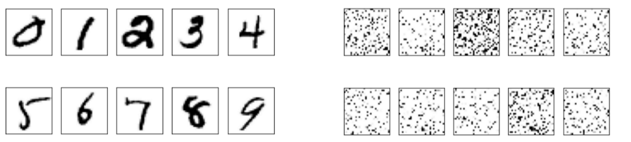
Consider now what that means visually. What you see in the above picture is a subset of the given images, and how they look like after generating a random reordering of the pixels and applying that reordering to each image.
Our visual system and brain model gets a near-100% accuracy on the original images. But if were to be shown reordered images like the ones on the right, most probably our accuracy rate would plummet to a baseline performance of 10% (random classification), even if we spend time 'training' with these images. On the other hand, our $C_{\mathit{good}}$ classifier is able to reach a 94% accuracy on such re-arranged images that have completely lost their original structure! This shows how impressive neural networks can be.
On the other hand, we would like to come up with an artificial neural model that will reach performance similar to ours on the 'structured' image data. This provides the motivation for Convolutional Neural Networks, special architectures that were designed to leverage the structure of image data.
19.3 The Hidden Feature vs the Hidden Image ⬤ 
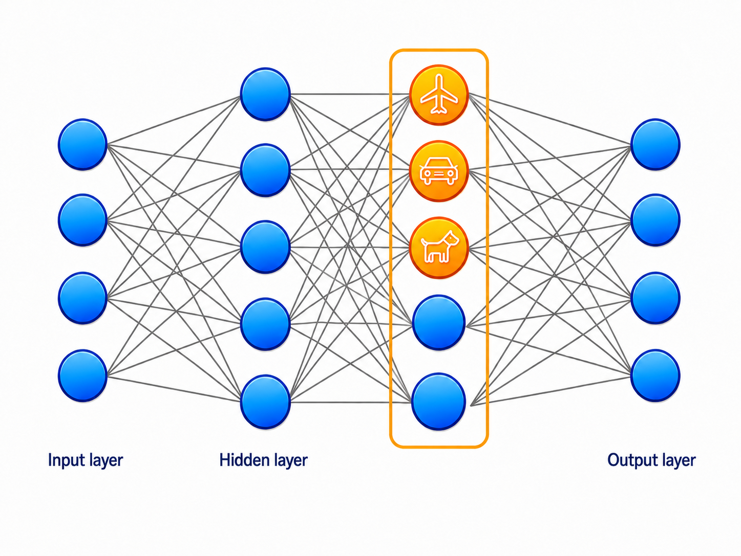
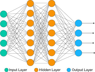
Recall that we can view the hidden neurons of a neural network as learned features. A single hidden neuron corresponds to one such feature and, as such, it is a global feature because its calculation depends on the entire input.
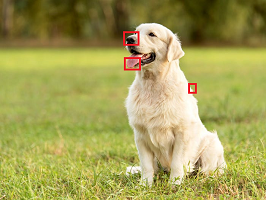
When looking at images, we do want to extract global features from these pictures, so as to (for example) determine if the picture contains some type of animal, object, or social media influencer. But before we make such global determinations, our eyes automatically scan the images for local features, such as contrast-based transitions between different objects in the image, or (as in the image above) tongues, ears, noses etc. In fact, we look for such local features everywhere in the image.
In this way, via an application of a filter, any given image can be mapped to another 'image' that encodes the presence of certain features in the input image.
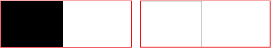
For example, consider the above two images. On the left side, we have a black and white image. We can apply a simple local 'filter' in every position of that image: if a black pixel has a neighboring pixel that is white, then we make it black; otherwise, we turn it white. Applying this local feature everywhere on the left image, we get the image on the right that encodes the 'edge' features of the input image.
Thus, the analogue of the single neuron that computes a global learned feature is a single trainable feature map that learns an array of features.
19.4 Calculating a Feature Map ⬤ 
Let's now show the application of a feature map in a mathematically more concrete way.
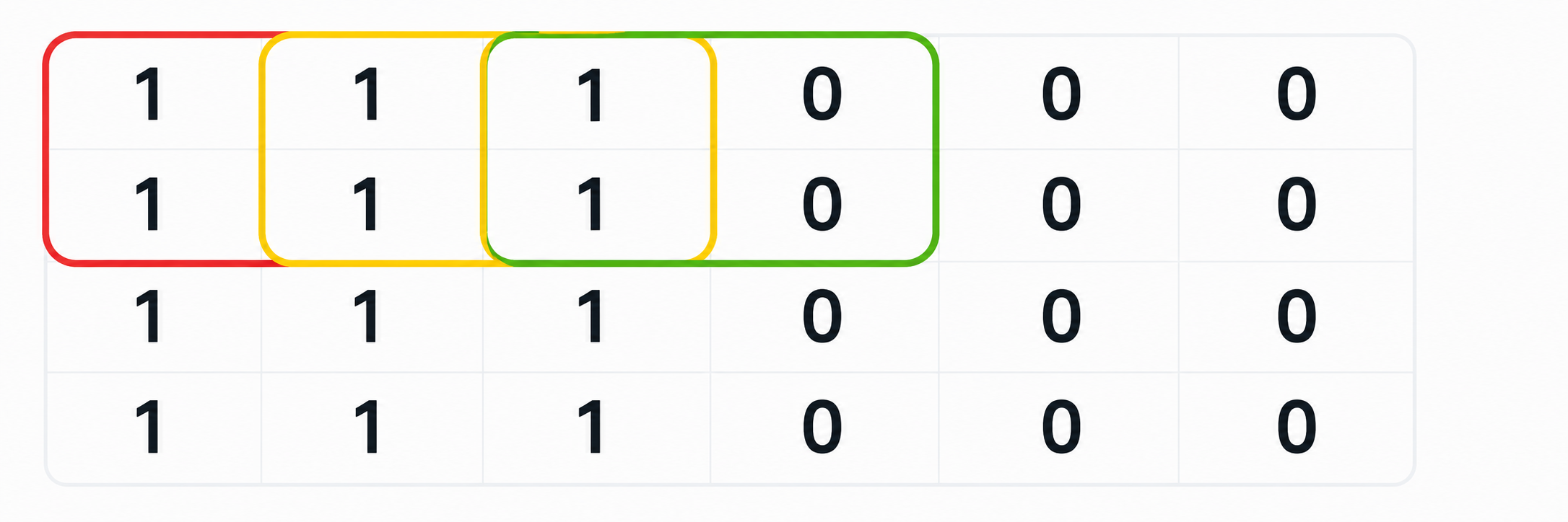
The image above is a miniature version of the black-and-white image of the previous section.
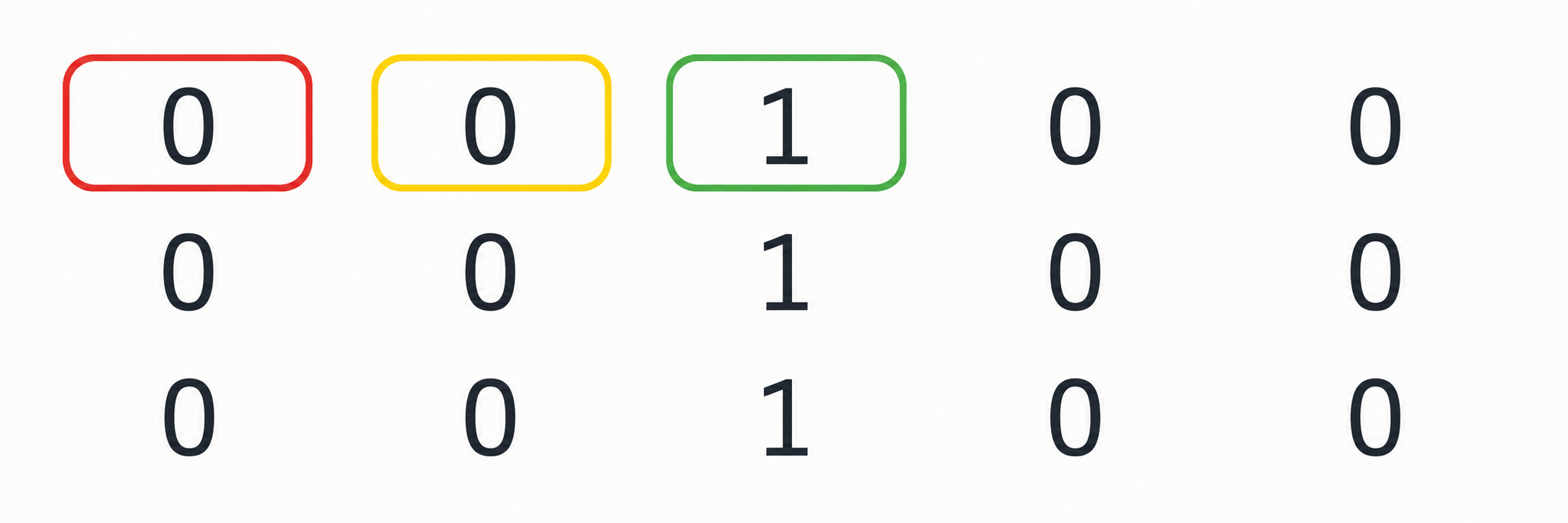
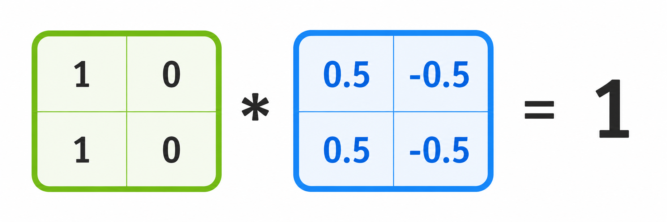
We can define a 2x2 filter as shown in blue above. The filter is applied to every 2x2 patch of the input image; the picture shows the application on the green patch. The output of a single application on a 2x2 patch is the sum of the entry-wise products of the input patch with the filter, i.e. a generalization of the inner product to 2D arrays.
We can then move the filter over all possible locations in the input image, and for each such location calculate a single output number, that is put into the corresponding location of the output feature map. This is illustrated in the above image, where we now see that applying this very simple filter results in an image that, as expected, has only a black column of pixels highlighting the 'edges' of the input image. Here we also observe that the output array is smaller by one unit in both dimensions.
19.5 The 2D Convolution ⬤ 
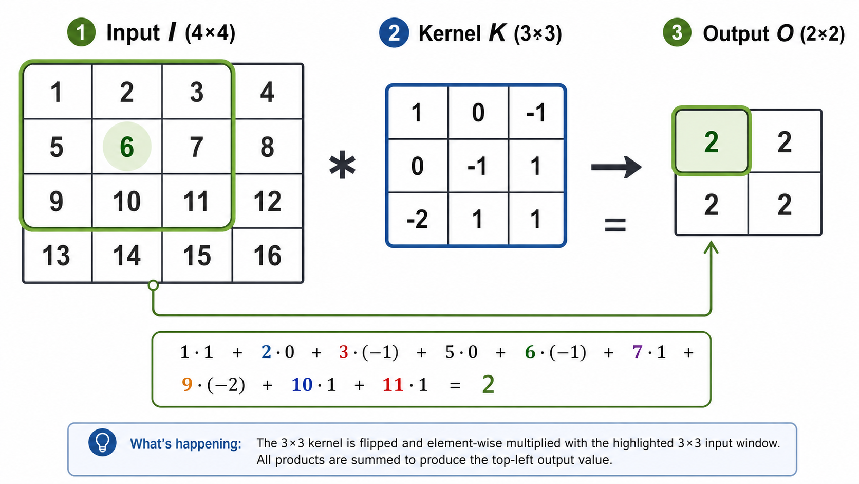
The operation we saw in the previous section is known as the 2D convolution. Here is one more example with a 3x3 kernel. We often use the '*' operator to denote the convolution between an array and a kernel, as shown below.
The 2D convolution is a linear operator on the input, because each part of the output is a linear combination of the entries of the input. In general, the convolution filter does not have to be square — it can have any rectangular dimensions.
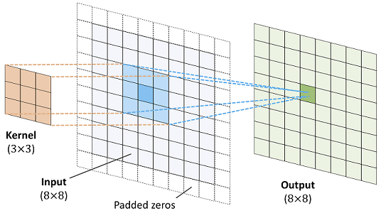
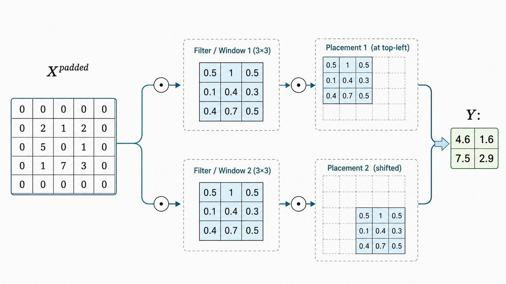
If we apply a $d\times d$ convolution on a $h \times w$ array, then the output array will have dimensions $(h-d+1)\times (w-d+1)$, and thus the output will be in general smaller. We often want the output array to retain the input dimension. In that case, we use padding, i.e. add an extra border of zeros around the input array, and we apply the convolution on that padded input, resulting in the appropriate dimensions in the output. This is illustrated in the picture below.
Standard implementations of 2D convolutions (e.g. in PyTorch) have two default modes of padding, 'valid' which essentially means no padding, and 'same' which internally applies the appropriate padding in order to retain the input dimension in the output.
An additional hyperparameter of 2D convolutions is the stride, which is a pair of numbers $(s_v,s_h)$. This is illustrated in the picture below, where the stride is $(s_v,s_h)=(2,2)$. The application of the kernel starts by placing its top-leftmost cell at the top-leftmost cell of the (potentially padded) input, which has coordinates $(0,0)$. Then, the possible locations of the top-leftmost cell of the kernel are positions of the form $(s_v\cdot i,s_h\cdot j)$ on the input, for all $i,j$ which allow the kernel to still fully fit in the input. This essentially means that we start with the kernel window at the top-leftmost position and then we slide it horizontally or vertically only by the increments specified by $(s_v,s_h)$.
In most cases $s_v$ and $s_h$ are equal, so we can specify the stride with only a single number $s$. The use of stride implies that we want to make the output dimensions smaller by a factor of $s$. And in many cases $s=2$, which means that the output will have dimensions approximately half of the input dimensions. For that reason the option of 'same' padding is not available in combination with the use of stride.
19.6 The Convolution Layer ⬤ 
We are now ready to discuss the convolutional layer. A linear layer in a standard neural network takes as a basic input a vector, and transforms it into another vector via the transformation $(xW^T+ b)$, where $W,b$ are trainable parameters.
19.6.1 Tensors and Channels
In the case of a convolutional layer the input is a set of 2D arrays, that can be viewed as different channels of the same image. These can be color channels, but also other types of channels that have been calculated in previous layers of the network. These channels of 2D arrays can be represented as a 3-dimensional array, that is more commmonly called a 3D tensor. So, the basic input of a convolutional layer is a 3D tensor.
The output of a convolutional layer is also a 3D tensor, a collection of channels, each of which is a 2D array. The number of output channels is a hyperparameter.
19.6.2 Example: One Output Channel
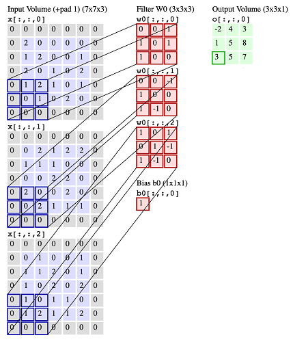
Let's now look into the case when we have $c_{\mathit{in}} = 3$ input channels and $c_{\mathit{out}}=1$ output channel. In the picture below, the 3 input channels are blue, and in this case they are padded. Then, the layer includes $c_{\mathit{in}}$ kernels along with a specification for the stride. In this case, the kernels are shown in red, and the stride is $(2,2)$. The kernels are in 1-to-1 correspondence with the input channels. Each kernel applies to the corresponding input and the result of the 2D convolution gives an output for that channel. Finally, these $c_{\mathit{in}}$ outputs are summed up, the same bias (a single scalar) is also added in every entry, and that results in the single output channel (shown in green).
In a convolutional layer, the filter weights and the bias will be trainable parameters. For example, in this case we would have $27+1$ parameters to learn.
Symbolically, if we let $I_1,I_2,I_3$ be the three arrays in the input channel, and $W_1,W_2,W_3$ be the 3 filters, then the input can be viewed as a 3D tensor $[I_1,I_2,I_3]$, the parameters can also be viewed as a 3D tensor $[W_1,W_2,W_3]$, and the operation gives the output $[W_1*I_1+W_2*I_2+W_3*I_3+b]$, where '*' is the convolution operator. The output in this case will also be a 3D-tensor, which in the example below will have dimensions $(1,3,3)$. (Note: The number of channels in these images is shown as the 3rd dimension of the tensor, but in implementations it is usually the 1st dimension).
19.6.2 Example: Two Output Channels
Let's now consider what happens when the number of output channels is $c_{\mathit{out}}=2$. This is a simple generalization of what we described in the case $c_{\mathit{out}}=1$: We define another set of $c_{\mathit{in}}$ filters and a new bias, and we apply them independently in the same fashion on the input channels, to calculate the second output channel. This is illustrated in the picture below.
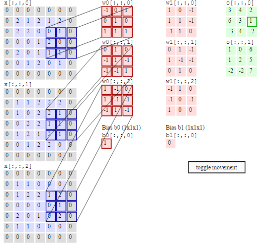
These operations generalize in the obvious way for arbitrary $c_{\mathit{in}}$ and $c_{\mathit{out}}$. When the kernel has size $w \times h$, the total number of parameters of a convolutional layer is $c_{\mathit{in}}\cdot c_{\mathit{out}} \cdot (w\cdot h +1)$.
The convolutional layer is linear.
Non-linearity: In standard ANNs, a linear layer is usually followed by an activation function $\phi$ — that is, we compute $\phi(xW^T + b)$. The same applies for convolutional neural layers: a nonlinear function (such as ReLU) is applied to each entry of the output arrays.
19.7 The Pooling and Dropout Layers ⬤ 
19.7.1 Pooling
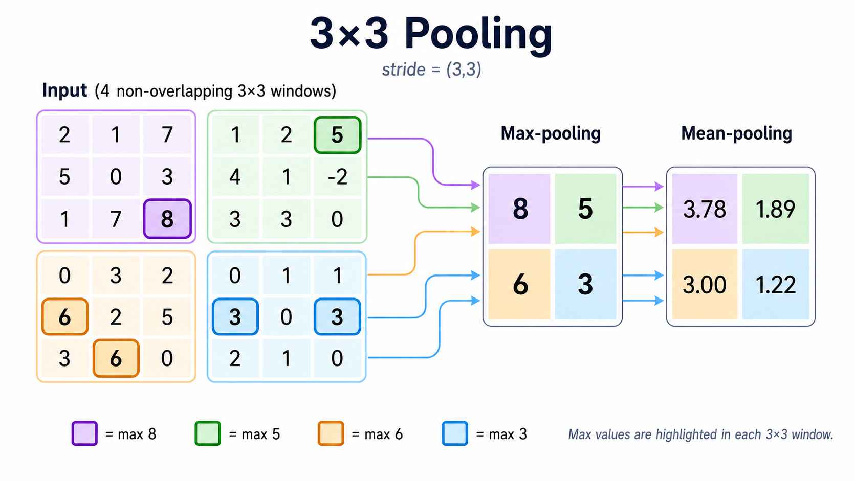
The mean pooling (or average pooling) operator takes as input a 2D array $I$ and returns another 2D array $O$. It operates on $I$ in exactly the same way as a kernel, except that all weights in the kernel are set equal to $1/T$, where $T$ is the total number of cells in the kernel. Importantly, these weights are always the same, and are not trainable. It is also usually the case that mean pooling is used in combination with a stride. Effectively, the mean pooling operator takes one image $I$ and 'summarizes' it into a smaller image $O$. Each 'pixel' in $O$ is an average of a patch of pixels in $I$.
The max pooling operator works in a similar way as mean pooling, except that it calculates the maximum over each patch, instead of the average.
The pooling layer. In a pooling layer we will have $c_{in}$ arrays in the input. The pooling layer applies the specified pooling operator on each input array, and outputs exactly $c_{in}$ arrays. Since pooling layers are used with stride, the output arrays are in general expected to be smaller relative to the input (often by a factor of 2 in each dimension).
19.7.2 Dropout
The dropout layer applies during the training process only to the activations $a_l$ of a previous 'regular' layer $l$ of the neural network. For each given minibatch in training, we replace the tensor of activations $a_h$ by $a'_h$, where a proportion $p$ of the entries in $a_l$ are randomly zeroed out, and the remaining entries are multiplied by $1/(1-p)$. Then $a'_h$ is used to compute the next layer. During testing the neural network uses all activations and learned weights.
This is illustrated in the picture below.
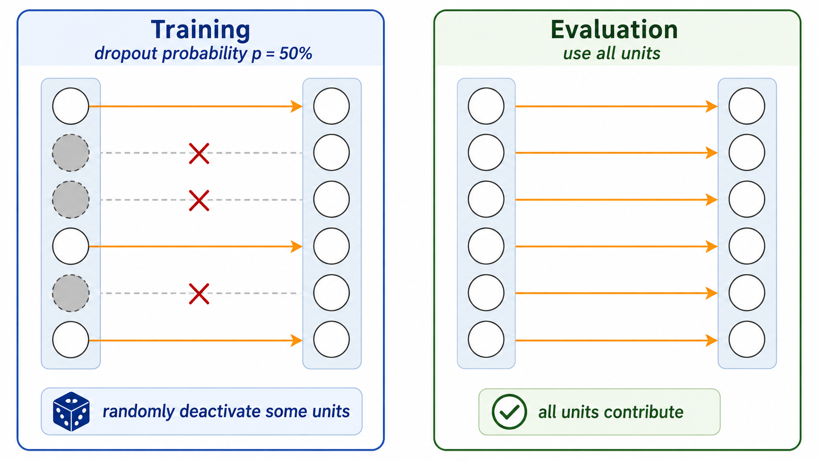
Dropout layers have been proposed to reduce overfitting, and improve generalization. They are widely popular, and have become the default mechanism currently used for regularization in deep neural networks.
19.7.3 A CNN architecture
We are now ready to look at a simple CNN architecture. This example is designed for the MNIST dataset, and is relatively small and shallow. Many other CNN architectures have been proposed. The diagram below shows how a single input 'point' propagates through the network. Here the point is a 3D tensor with only one color channel. If we wanted to handle 3 color channels, we would simply change the appropriate dimension of the input channel to 3. (Note: In implementations, the number of channels is usually the 1st dimension, not the 3rd dimension as shown in the diagram.)
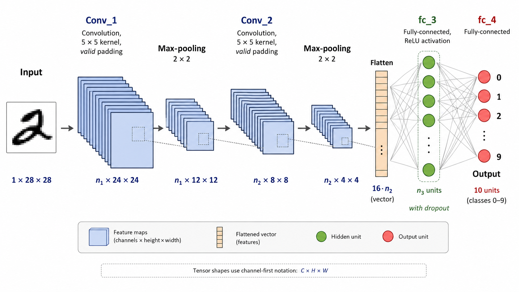
Here are some observations drawn from the above illustration.
The 3D tensor moves first from the input to the first hidden layer, by applying a number of learnable convolution filters of size $5\times 5$. In this case, the number of output channels $n_1$ is a hyperparameter. That means that the number of hyperparameters is $1\times n_1 \times 26$. Even for a large number of output channels (e.g. 100), this number is relatively small, so we can afford to learn multiple different types of local feature maps.
Then the tensor of all these $n_1$ feature maps goes through a pooling layer which is used with a stride of 2. That reduces the dimensions of these arrays by 2.
Then again we have another convolutional layer. Because now the arrays have a smaller size, they don't take up as much memory space, so we can afford to learn even more feature maps $n_2$. The number of parameters here will be higher, $n_1\times n_2 \times 26$, but this is still not too big, the important thing is that these tensors fit in the memory.
Finally we have another pooling layer.
It is important to remember that after each convolution layer we apply a non-linear activation function, usually the ReLU.
The $n_2$ array features after the last pooling layer have a total of $16\times n_2$ entries, that we then flatten into a vector. After that point we have a standard ANN, with an additional dropout layer. The last layer is a softmax with 10 outputs because we have a 10-label classification problem.
It is also interesting to think about the receptive field of each pixel in the hidden layers. In the first hidden convolutional layer, any given pixel is a local feature of a 5x5 patch of the image. However, due to the pooling layer which summarizes 4 pixels into 1, the second convolutional layer pixels depend on a larger patch of the image. That reflects our intuition that we humans scan an image at multiple layers of resolution in order to 'see the global picture'.
19.7.4 Training Backpropagation
The above describe how the CNN operates in the forward mode, and specifically on a single point. When training with minibatches the layers process 4D tensors, where the outer dimension corresponds to the batch size $\mathit{bsize}$. For example, in this case we would have input tensors of size $(\mathit{bsize},1,28,28)$.
In the forward mode, the network calculates the loss function parameterized by the weights in the kernels and final MLP layers. As usual, the network then computes derivatives and performs backpropagation to update the weights.
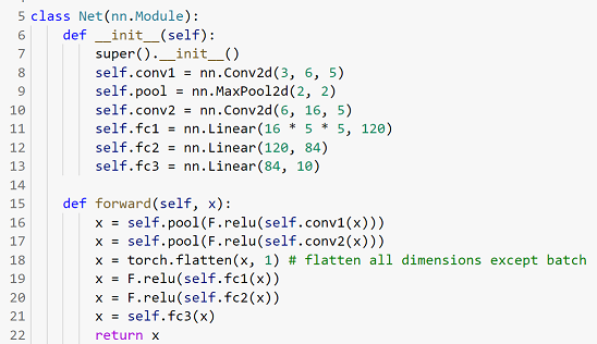
19.8 CNNs with PyTorch ⬤ 
Here is the code notebook.
This is how the code for a similar architecture looks in PyTorch. Despite the fact that this code handles 4D tensors (minibatches), it is conceptually easy to understand and map back to the architecture, as the minibatch dimension is handled implicitly. The only point where we must be aware of the minibatch dimension is in the flatten layer at Line 18, where now the features of the batch of size $\mathit{bsize}$ are flattened into an array (and not a vector), with each row corresponding to the flattened features of one point in the batch. This is done by flattening all dimensions except the first. For each tensor in this 4D batch, the procedure flattens it separately into a single vector.