Module 20 — Recurrent Neural Networks
20.1 Predicting the Future ⬤ 
The ability to accurately predict the future can be extremely valuable. One example is in the stock market.
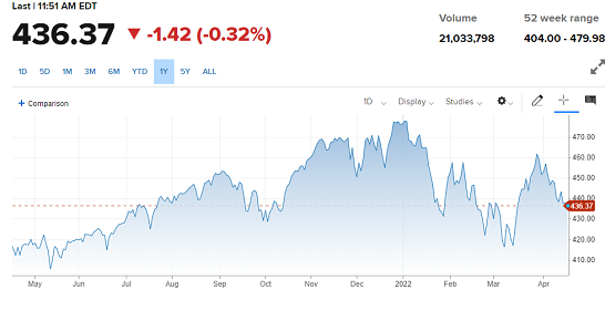
Predicting the future based on past data relies on the assumption that the next value in a timeseries can be at least partially predicted based on the recent history and all available data.
Given the tools we have learned so far, it is not very difficult to design a model that attempts to predict the value of a stock tomorrow (regression), or perhaps whether it will go up or down (classification). For this, we would need access to effective features, and their corresponding labels, and then use a regressor or classifier. For example, we could use the history of the last 20 days, and record 5 values each day: [open, close, low, high, volume]. That would give 100 features. Then we can go back in history, find many 20-day windows, use the history of the next day as our label, and train our favorite model. This could work, especially if we are able to 'mine' or engineer the appropriate features. However, it is clear that these vectorized features do not retain the underlying temporal information which, intuitively, should be taken into account.
This motivates the design of neural architectures that are able to natively work on sequences of data. And that is precisely what Recurrent Neural Networks are.
While one might question whether actionable predictions can be made for the stock market, it is certainly the case that predictions are possible when it comes to weather forecasting, which itself is an extremely valuable task.
Weather prediction has been getting progressively better as physical models, algorithms and hardware improve. Traditional weather forecasting is based on equations that take as input the present conditions, and then make near-term predictions with high accuracy, albeit always involving some uncertainty. These models output a range of possible near-term predictions, rather than just a single prediction. These near-term predictions are fed back into the model to make longer-term predictions, in an autoregressive fashion.
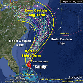

To make this more precise, suppose that the model uses a window of $t$ days $[1,t]$ to make a prediction for day $t+1$. Then that prediction can be used to define another window of $t$ days: $[2,t+1]$. That can be in turn used to make a prediction for $t+2$, and following that autoregression procedure, we can make a longer-term forecast. Of course, because we really have a set of predictions for $t+1$, each of them will produce a set of predictions of $t+2$, and so on. This gives rise to the familiar hurricane 'cones of uncertainty' based on running multiple simulations and sampling many different trajectories of the autoregressive forecast.
Weather forecast is a topic where ML-based techniques can bring further progress. Indeed, it was recently announced that deep models have reached the highest known accuracy in 'nowcasts', i.e. very near-term forecasts with good localization [1].
Many other types of data come naturally in sequence form. Natural language and music are important examples.
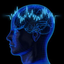
20.2 Recurrent Neural Networks: Biological Intuition ⬤ 
After a trained neural network has processed one point, all activations of the neurons are thrown away.
However, when our brain processes an auditory signal, or even written natural language, our mind state is updated not just based on the current input only, but also based on previous states. In this way, we continously combine external input with those of our previous neural activations that provide the context for understanding what we hear.
This idea — the use of a hidden state (the activations of the hidden layer) together with the next input of the sequence — is central to recurrent neural networks.
20.3 The Recurrent Layer ⬤ 
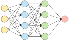
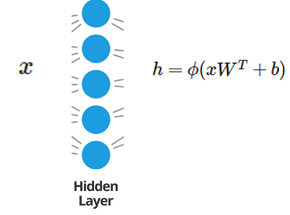
It is useful to think once again about how the simple (non-recurrent) hidden layer works. It takes as input a point $x$ and computes an activation as shown below. Afterwards, the activation then is discarded; that is, the neurons are memoryless.
The hidden recurrent layer does not forget its intermediate activations while the network is processing a sequence. Consider for example the following illustration:
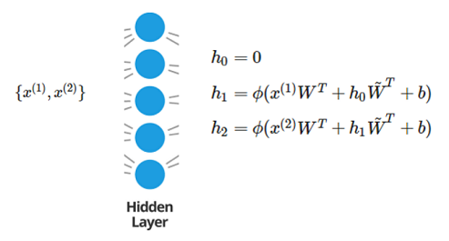
Initially the neuron's activations are $h^{(0)}=0$. Then, when the first point $x^{(1)}$ comes into the layer, the activation $h^{(1)}$ is computed as it would be in a regular neural network. However, the activation persists, and is reused when computing activations $h^{(2)}$, in combination with the input vector $x^{(2)}$.
The computation of $h_2$ involves multiplying $h_1$ with another matrix of parameters $\tilde{W}$. Observe that $\tilde{W}$ is a square matrix of dimension $k\times k$, where $k$ is the number of neurons in the hidden layer; on the other hand, $W$ has shape $k \times d$, where $d$ is the dimension of the input vectors. More generally, the activation at time $t$ is computed as follows:
$$h^{(t)} = \phi(x^{(t)}W^T + h^{(t-1)} \tilde{W}^T + b)\, .$$
The recurrent layer usually takes as input a sequence of predetermined length, $\{x^{(1)},\ldots,x^{(t)}\}$, and produces as output the sequence of activations $\{h^{(1)},\ldots,h^{(t)}\}$. The final vector $h^{(t)}$ can be viewed as the 'state of mind' when the entire sequence has been processed. Before the network starts processing a new sequence, the activations of the hidden neurons are reset to 0.
There is an alternative --and more computationally efficient-- way of computing the activations $h^{(t)}$.
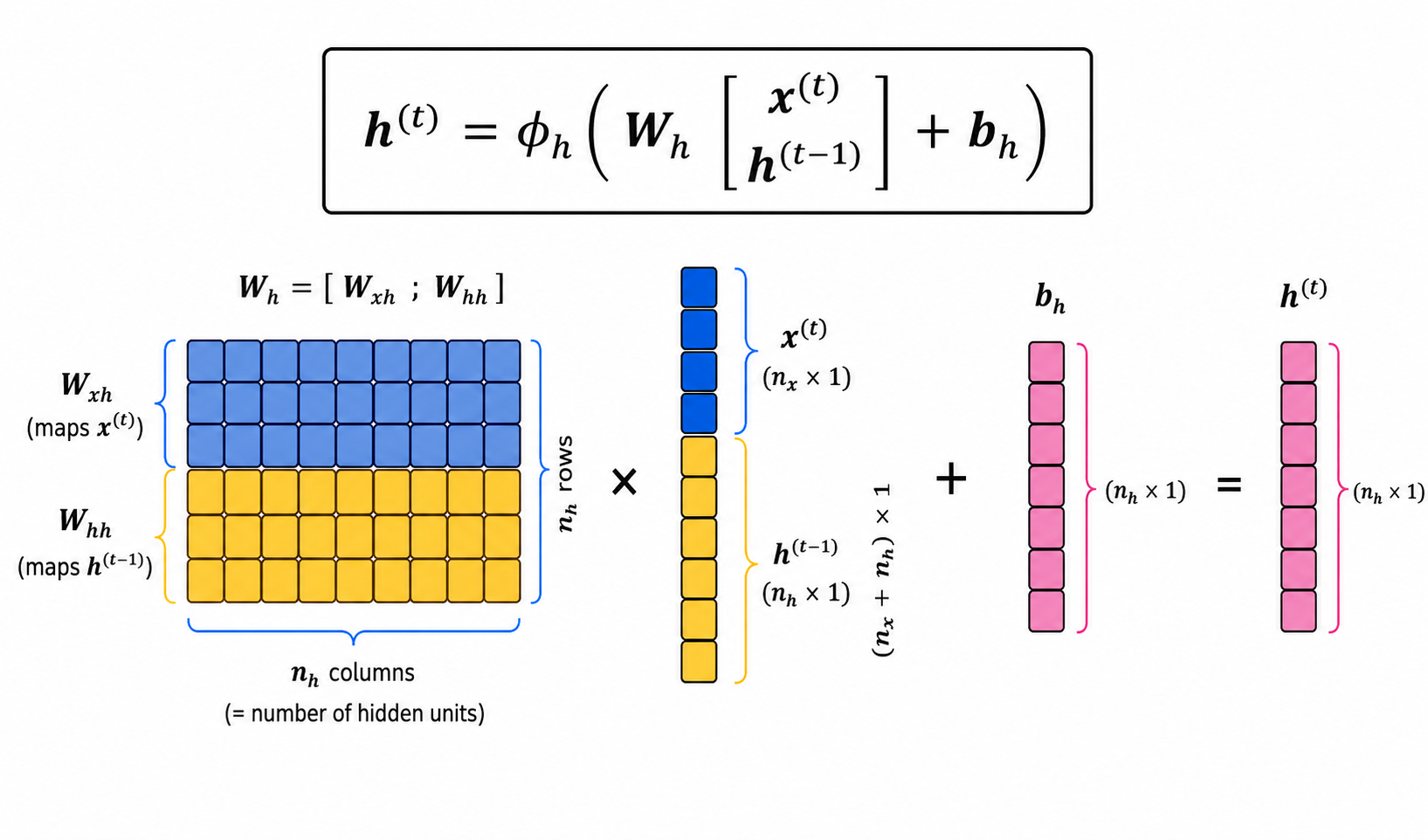
This is given in the picture above. The two matrices of weights are stacked together, and also $x^{(t)}$ and $h^{(t-1)}$ are stacked together. In that way the computation can be done with only one matrix multiplication. (Note: In this graphic we use column vectors instead of the usual row vectors for $x$ and $h$.)
20.4 More Recurrent Layers ⬤ 
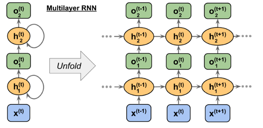
When we have more than one recurrent layer, we can simply think of them as illustrated below: The first layer takes as input a sequence of vectors and produces as output another sequence, that becomes the input for the second layer, and so on.
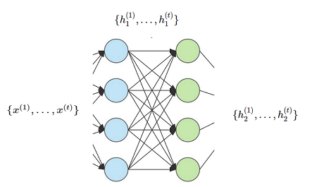
It is useful to look at the 'unfolded' picture of how the computation works internally in these two layers. The second layer does not have to wait for the entire output sequence from the first layer. Instead, when $h_1^{(t)} = o_1^{(t)}$ becomes available, it can start the calculation of $h_2^{(t)}$. Thus, the forward parallel calculation of $k$ recurrent layers on a sequence of length $t$ will take time proportional to $t\cdot T$, where $T$ is the computation time for evaluating these $k$ layers on a single point in a standard non-recurrent network.
However, the backpropagation through $k$ layers on a sequence of length $t$ would have $k\cdot t$ backpropagation steps — and consequently, the length of the sequence affects the depth of the network and the backpropagation calculation. The training of recurrent networks is therefore more of a computational challenge than for standard networks.
20.5 A Recurrent Neural Network and the Embedding Layer for NLP ⬤ 
We can now think of how to design an RNN for timeseries from the stock market, as discussed in section 20.1. We can simply define one layer to be recurrent, and we can now insert as input the sequence $\{x^{(1)},\ldots,x^{(20)}\}$ of 5-dimensional features of the time window preceding the target day. The hidden layer will output another sequence $\{h^{(1)},\ldots,h^{(20)}\}$, where $h^{(20)}$ encodes information from the entire window. We can then pass the single point $h^{(20)}$ to the next layer, and then finally propagate it through to the output layer that can be set to be a sigmoid for classification, or simply a linear layer for regression.
20.5.1 The Embedding Layer
But what about processing text and natural language in general? The input could be a sentence such as "I loved the earlier movies in the series, but not the last one", from which we would want to infer its sentiment. The problem is that, by construction, RNNs take as input a sequence of vectors and not a sequence of words. The solution is to use an embedding layer.
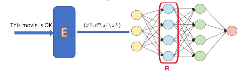
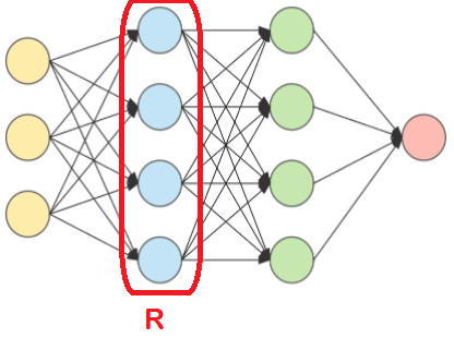
The embedding layer maps (or 'embeds') words in the vocabulary to $d$-dimensional vectors. One can think of the embedding layer as a matrix of parameters $W$ with shape $N\times d$, where $N$ is the size of the vocabulary and $d$ is the embedding dimension, which is a hyperparameter. The matrix $W$ is trainable inside this network, which means that we essentially learn vector representations for all the words.
We can train these embedding layers from scratch for any given application, but pre-trained embedding layers are often available for use in initialization, or even as fixed non-trainable layers.
20.5.2 The 'Magic' of Word Embeddings
It has been observed that learned word embeddings are linguistically meaningful. For example, if we look at the vector embedding $v$ of the word 'beautiful', then the nearest neighbors of that vector $v$ will likely be vectors corresponding to related words, such as 'pretty', 'handsome', and so on. Even algebraic operations make sense in practice: for example, if we take the two vectors $v_1$ and $u_1$ for the words 'France' and 'Paris', and then consider their difference $d=v_1-u_1$ that somehow encodes the notional difference between a country and its capital. So, if we take $v_2$ to be the vector for 'Italy', then $v_2 = v_1-d$ will give me a vector $u_2'$. That vector will not likely be corresponding directly to any word in the vocabulary. But if we check the nearest neighbors of $u_2'$, they would likely include 'Rome', with the vector $u_2$ for 'Rome' very often being the nearest neighbor to $u_2'$.
All recent advances in NLP derive from the power of word embeddings. It may be that internally, our brains also represent language as vectors!
20.7 Bidirectional Recurrent Layers ⬤ 
Consider the expression 'new year'. Our understanding of it allows us to imagine what the previous word might be: 'happy'. In some sense, that implies that our ability to predict the past implies a better understanding of the time sequence. That is also true in physics, where equations are time reversible and do give us the ability to back-calculate a previous state. This motivates the introduction of bidirectional layers.
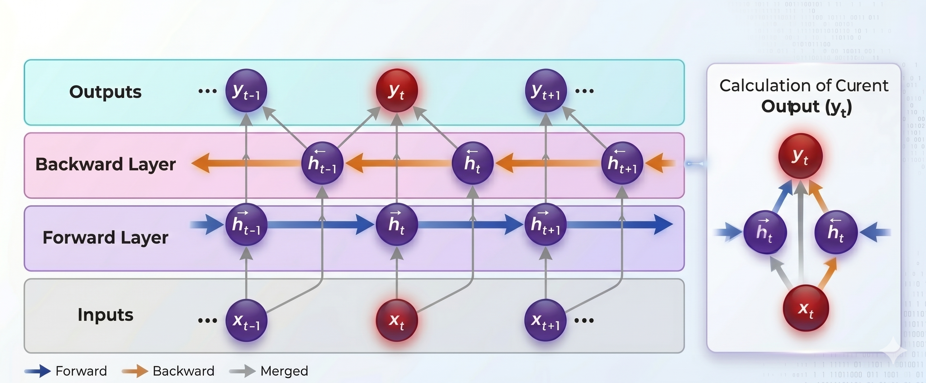
A bidirectional layer consists of two different recurrent layers, with different sets of parameters. The first layer works as usual, but the second layer reads the input sequence in reverse order. Thus, given an input sequence $\{x^{(1)}, \ldots, x{(t)}\}$, the first layer will output sequence $\{h_f^{(1)}, \ldots, h_f^{(t)}\}$, and the second layer will output a sequence $\{h_s^{(t)}, \ldots, h_s^{(1)}\}$. Then, the output sequence of the entire bidirectional layer will be: $\{y^{(1)}, \ldots, y{(t)}\}$, where $$ y^{(i)} = h_f^{(i)}+h_s^{(i)} $$
Alternatively, $h_f^{(i)}$ and $h_s^{(i)}$ can be concatenated. Thus the bidirectional layer outputs at time $t$ is a combination of the forward and the backward understanding of the sentence. This has proven to be an effective trick.
20.8 Newer Types of Recurrent Layers ⬤ 
The original recurrent layers have been vastly improved in recent years, resulting in better learning for deeper sequences.
Here let's see how 'Gated Recurrent Units' (GRUs) work.
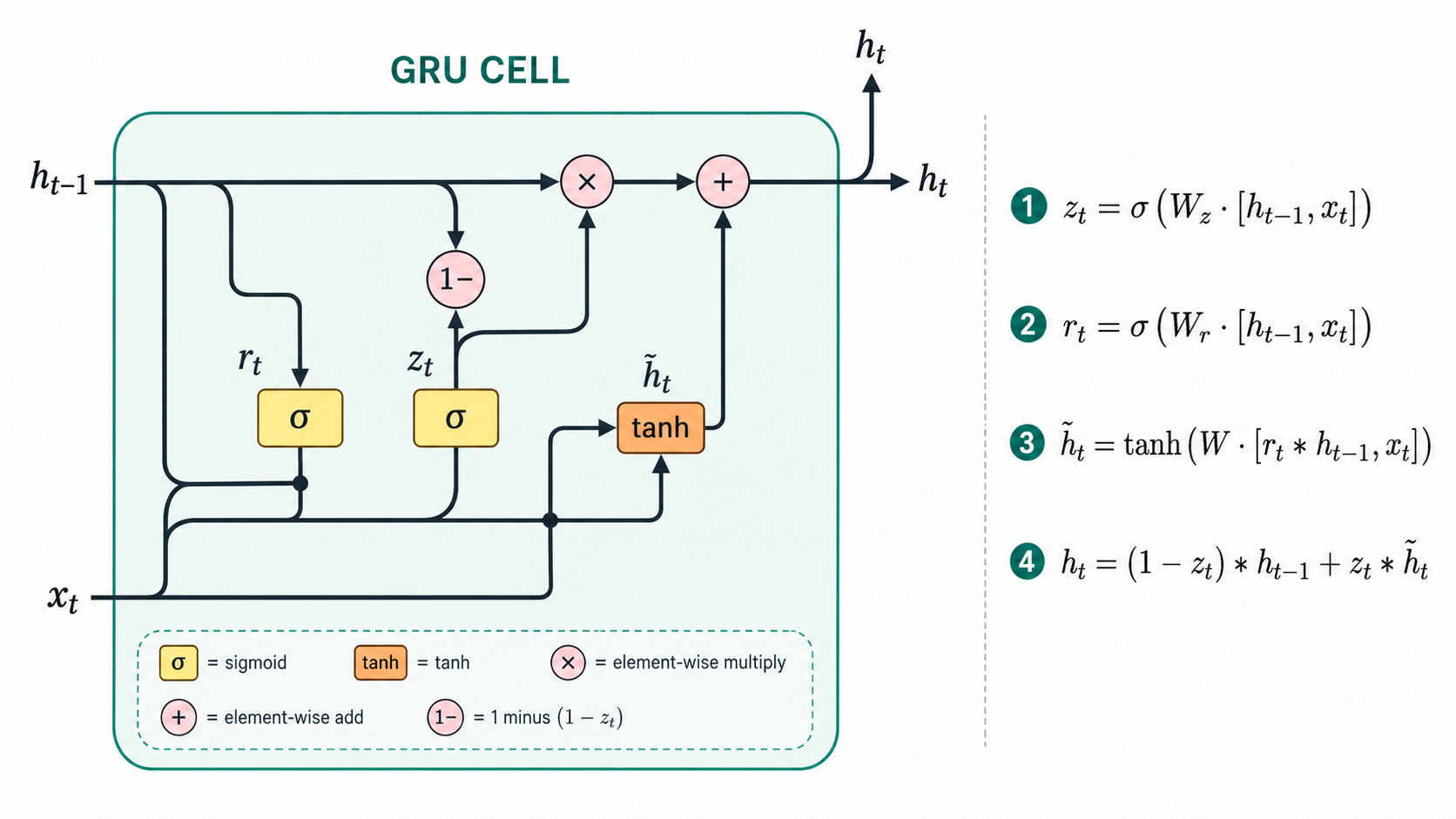
The main idea of the GRU gate is that the new hidden state $h_t$ is an update of the previous hidden state $h_{t-1}$. In that update, part comes directly from $h_{t-1}$ and the rest from a 'provisional' activation $\tilde{h}_{t}$. The update weights depend on a learnable set of weights that are different for each neuron. In that way, after training, the hidden layer can have neurons that are more or less sensitive to their previous hidden state.
The GRU also includes a reset mechanism which can learn to partially forget the previous hidden state of selective neurons before the calculation of the new provisional hidden state. This intuitively can be effective when we have abrupt changes in a sentence (e.g. a period), or in a time series (e.g. a large drop in stock value after earnings).
The above equations explain how $h_t$ is computed. In this picture $W_z, W_r$ are additional matrices of trainable parameters, and $r_t, z_t$ are vectors of dimension equal to $h_t$. Observe that $r_t,z_t$ involve trainable parameters, and that their activation is sigmoid, which means that they are numbers in $[0,1]$. Each entry of $r_t$ is the reset factor for the corresponding neuron, and each entry of $z_t$ is the update weight for the corresponding neuron. (Note: here, * denotes entry-wise multiplication, not convolution.)
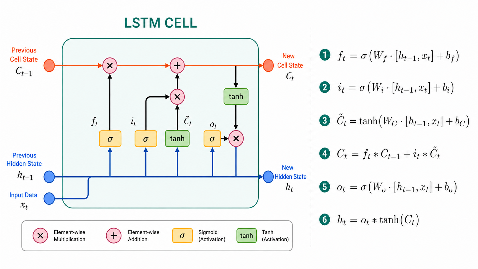
GRUs were preceded by LSTMs (Long Short-Term Memory), which have more trainable parameters than GRUs and used an extra 'memory' (cell state) vector besides the hidden state. In general, GRUs are considered more powerful. Here is what an LSTM looks like.
20.9 Character-Level Language Modeling ⬤ 
RNNs have been used for character-level language modeling, where the task is to predict the next character in a sequence of letters coming from an input text. Here is what this prediction problem looks like:
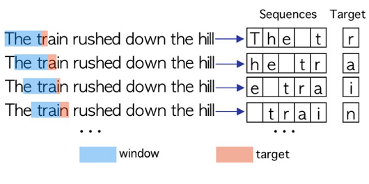
The question is, why should we bother training a model to do well on this? Fundamentally, the ability to predict some probabilities for the next character is closely related to language understanding: consider how difficult it would be to make any reasonable prediction for a text coming from an unknown language! So, models for character prediction can be regarded as stepping stones on the way to being able to design models that can 'understand' language.
We can also imagine practical auto-complete applications, similar to what happens when we type text in the query window of a search engine.
Character prediction models can also be used in the auto-regressive fashion we described in Section 20.1. We can start with a 'seed' text, and continue to generate letters hoping that the overall output will look like a reasonable completion of the seed text. Thus, such models can be used for language generation.
20.9.1 An Architecture
Here is one architecture for character-based language modeling, taken from here.
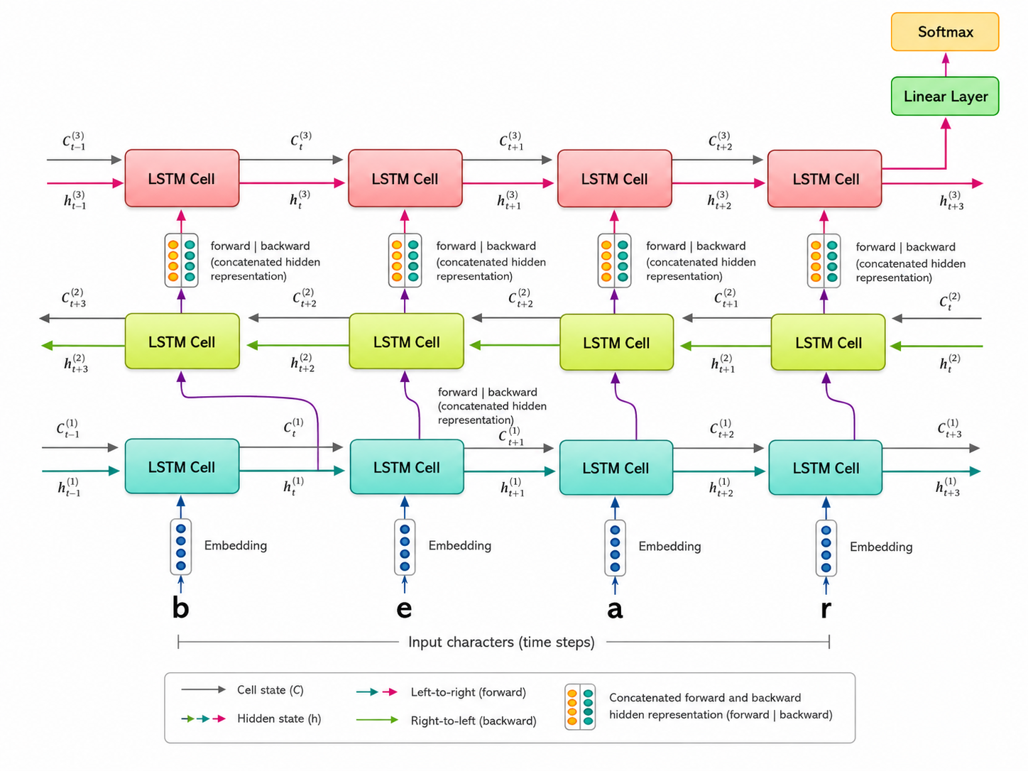
This is the 'unrolled' picture of the architecture, but we can see the basic elements. There is still a learnable embedding layer for converting characters to vectors. Next we have a bidirectional LSTM layer, with concatenation of the outputs of the forward and backward layers. These are passed into a unidirectional LSTM layer. That produces an output sequence, of which we keep the last vector, that we then feed to a linear layer, and finally to the final softmax layer. The last softmax layer must have 26 outputs, since we are trying to predict the next character.
Such architectures reach a decent accuracy for predicting the next character, depending of course on the length of the training window and the amount of data.
20.9.2 Generating Text
This is how text generation works on this toy architecture and dataset:
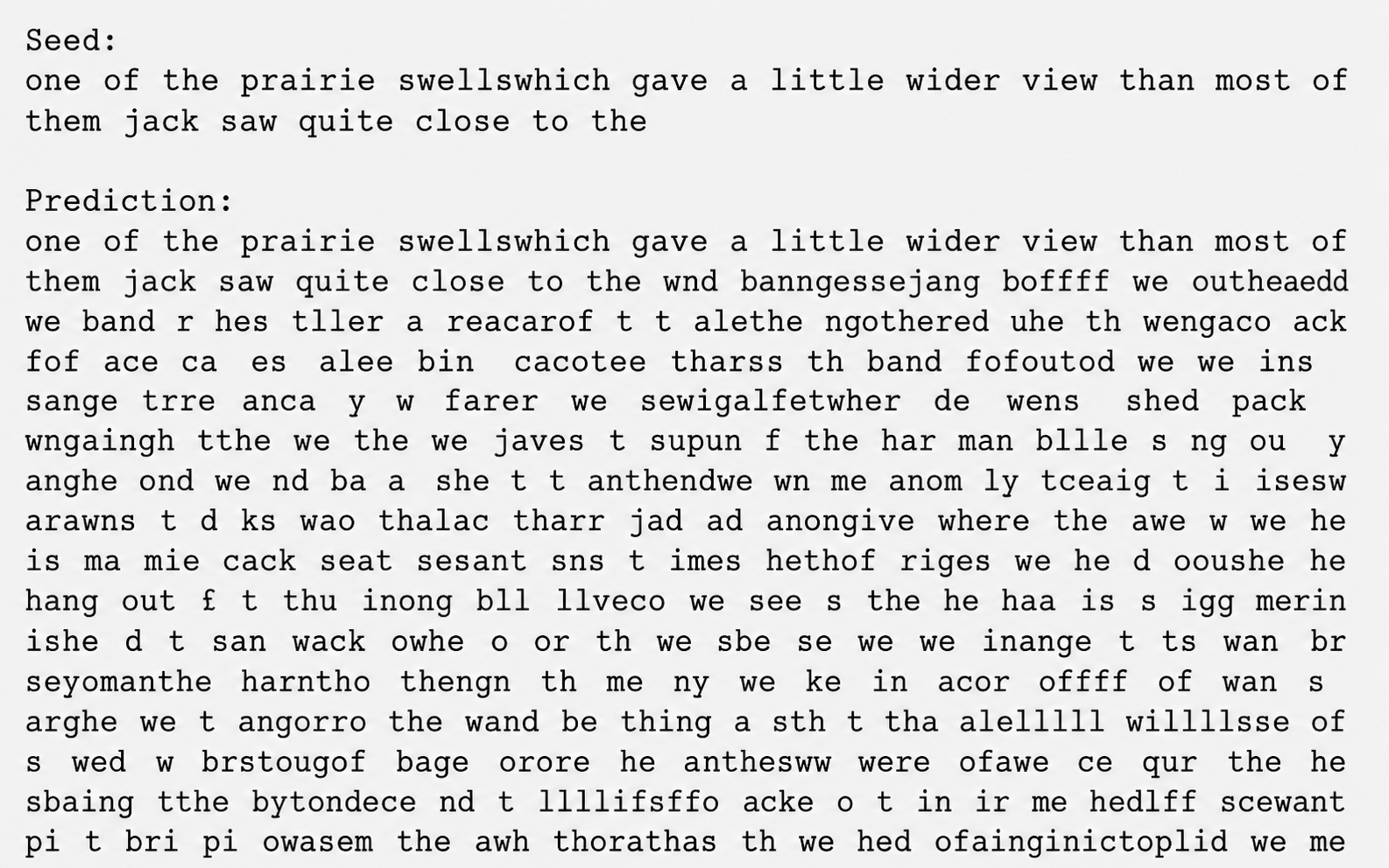
The performance is not so great, but more complex models have reached interesting levels of coherent text generation. It should be noted that because the softmax of this model predicts only a probability for the next letter, when generating text that letter is not selected deterministically, but instead at random with some probability. Therefore, many different texts can be produced from a given seed. Skewing the selection probabilities can yield more coherent and reasonable texts.
20.10 The Promise of Deep Learning ⬤ 
More sophisticated deep models and techniques can reach remarkable performance in generating sequences like text and music. The world has already its first AI composer [2].
References
[1] Nowcasting the next hour of rain, DeepMind blog.
[2] AIVA, The Artificial Intelligence composing emotional soundtrack music.