Module 3 — Linear Regression, Gradient Descent and Feature Engineering¶

3.1 Parametric Learning ⬤ ¶

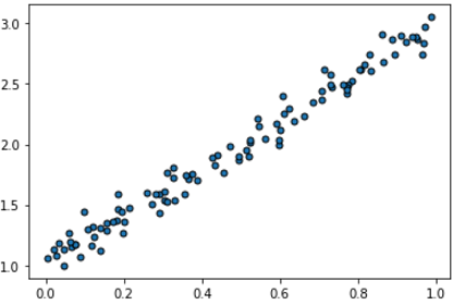
We now consider a simple supervised regression problem. The data matrix $X$ has dimension $n\times 1$ and the labels matrix $y$, also of dimension $n\times 1$ contains numerical entries. These pairs $(X_i,y_i)$ are visualized in the following picture. This is a very special 1-dimensional example that we will generalize later.

Noisy linear function

Goal. We want to find a relatively simple and concise 'law', i.e. a function $y=f(x)$, that describes the data as well as possible. Recall that an 1-NN algorithm can always return precisely the correct label for each point $X_i$ in the given data set $X$. In this case, because we want the function to be relatively simple, it is unlikely that we can find an $f$ such that $y_i$ is exactly equal to $f(X_i)$ for all points $X_i$. We will instead aim to find a function such that $f(X_i)$ is - in some sense - a good approximation to $y_i$. The intuition is that such a function $f$ can then used to give predictions for the numerical labels of unseen points.

Modeling the data. Data often contains some natural variability, possibly due to measurement noise etc. The given data appear to approximately follow a line with some added variability. So, we can use our intuition and model the data as a line; that is, we assume that the function is the form of a line: $$ y = ax+b\, . $$

Here $a,b$ are unknown parameters. The equation $y = ax+b$ is thus a set of infinitely many hypotheses, or models for the 'law' that generates data, and we want to find values for $a$ and $b$ that give the best possible hypothesis or model - that is, the model that gives the best approximations $f(X_i)$ for $y_i$.

Data modeling has its origins in Statistics. Indeed, Machine Learning is historically rooted in Statistics. The material of this section predates Machine Learning by many decades, or even centuries. But it is in the core of nearly all algorithms in current ML and Deep Learning.

3.2 Loss Function ⬤ ¶

Suppose we have now fixed a model $f$. It is not too difficult to quantify the error of approximation on a single data point $X_i$: $$ e_i = |f(X_i) - y_i| $$

We can extend these individual errors to a global error, that we will call the loss function, defined as follows: $$ L = \frac{1}{n} \cdot\sum_{i=1}^n e_i^2 $$

With this definition, $L$ is often called the mean squared error. When $L$ is small we expect that most individual errors $e_i$ will also be small. So, it makes sense to find a model $f(x) = ax + b$ that yields a small loss $L$. Recall that $X$ and $y$ are given to us, so $L$ only depends on the choice of $a,b$. We will sometimes write $L(a,b)$ to emphasize that.

3.2.1 Why MSE?¶

There are potentially many ways to define a global loss. For example, we could have picked the much simpler function $L = (1/n) \sum_i e_i$, or even $L = max_i\{e_i\}$. MSE is a popular choice, though, mainly due to its nice mathematical properties.

~ Convex function illustration

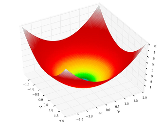
This 3D plot demonstrates these properties. Here the two axes correspond to the variables $a,b$ and the third axis corresponds to $L(a,b)$. Its characteristic shape illustrates that the function is convex, and as such, it has a unique local and global minimum. In other words, there is a unique setting of $(a,b)$ that minimize the loss. A general way to think about the minimum is this: For each value $c>0$ there is a set of points $(a,b)$ that satisfy $L(a,b)=c$, and that set is called a function level set - in the above 3D plot all points in a level set get precisely the same color. The level set for $c=0$ is a unique point.

The function is also smooth, or 'differentiable' at any point $(a,b)$. And that brings us to calculus.

3.3 Gradient Descent in a Nutshell ⬤ ¶

3.3.1 Gradient Descent in One Variable¶

Consider a simple function with one variable $y=x^2$ (by the way, these $x,y$ have nothing to do with our model $y=ax+b$, we are just reusing symbols).

Quadratic Function

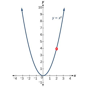
You may recall from calculus that the derivative of this function is $f'(x) = 2x$. By its definition, the derivative at some point $x$ gives us the rate at which the function changes. Moreover, the sign of the derivative tells us whether the function is locally increasing. As an example, at point $x=2$ we get a positive derivative of 4, which means that the function is increasing as $x$ increases. On the other hand, the derivative at $x=-2$ is equal to $-4$, which means that the function is decreasing.

If we then want to nudge our point $x$ towards the minimum of the function we can do an update of the following form: $$ x \leftarrow x - \rho \cdot \mathit{sign}\,(f'(x))\, , $$ where $\rho$ is a step size. We can carefully check and see that independent of whether the derivative has a positive or negative sign, if $\rho$ is sufficiently small, the updated $x$ will be closer to the minimum of the function.

A good $\rho$ should depend on how fast the function changes, i.e. in the derivative itself. It is then more natural to make $\rho$ independent of the derivative and use the following update rule: $$ x \leftarrow x - \rho \cdot f'(x)\, . $$

This update steps can be repeated multiple times to bring our point $x$ closer to the minimum. Because these iterative updates nudge our point to descend towards the minimum, and we use the derivative (the gradient for one dimension), we call this update process gradient descent.

Exercise: Think about the effect of picking a step size $\rho<1$, or $\rho>1$, or $\rho=1$.

3.3.2 Partial Derivatives¶

Consider now a 2-variate function, e.g. $f(a,b) = a^2+3ab+b^2+3$. One can use partial derivatives to get information about the speed of the function in each coordinate/axis separately.

For example, we can consider $b$ as a fixed number, and compute the partial derivative of $f$ with respect to $a$:

$$ \frac{\partial f }{\partial a} = 2a + 3b \, . $$

3.3.3 Gradient Descent in Multiple Dimensions¶

Suppose now we have a fixed point $(a,b)$ and we want to nudge it towards a minimum of the function $f(x,y)$. This can done by finding the update rule along the $x$-axis only, as if $b$ was fixed, and vice-versa. This gives us two different single-variable update rules:

$$ a \leftarrow a - \rho\,\frac{\partial f}{\partial a}\, , $$ and $$ b \leftarrow b - \rho\,\frac{\partial f}{\partial b}\, . $$

As it turns out, applying both these updates nudges our point $(a,b)$ to the direction of the fastest descent towards the minimum, and for a sufficiently small $\rho$, the point indeed moves closer to the minimum.

Again, gradient descent is the iterative application of multiple such update steps, one along each axis.

The same exact logic applies for an arbitrary number of variables, i.e. dimensions.

3.4 Gradient Descent as a Learning Algorithm ⬤ ¶

Recall that we are seeking to find a model that minimizes our loss function $L(a,b)$. Minimizing $L(a,b)$ can be done in many ways. However it will be helpful to consider two characteristics of human learning:

We learn from mistakes that nudge our plastic brains to adapt and become better at various tasks. For example, when we learn how to speak we make multiple mistakes that are corrected by our parents and guardians.
There is a saying that "repetition is the mother of learning". Indeed, in order to learn, we may cycle through the same (or similar) mistakes a number of times in order to correct them, or to minimize our errors.

This suggests that among all possible ways of minimizing the error $L(a,b)$, gradient descent may be the algorithm that most closely resembles the intuition we have about ourselves.

The constant $\rho$, that we called the "step size", can be also thought as a learning rate that determines how fast we adapt to the errors we make. Reflecting again about ourselves, we know that humans lose some of their flexibility and quick adaptability as they mature. And while maturity may not always be a great thing, it may be a necessity for better learning.

3.5 Gradient Descent for MSE ⬤ ¶

Let's go back to our MSE loss function $L(a,b)$, and try to make the update rules of gradient descent more specific to it. Recall that

$$ n\cdot L(a,b) = e_1^2 + \ldots + e_n^2\, , $$ where $$ e_j = |f(X_j) - y_j| = |a X_j + b - y_j|\, . $$

That is, we have one error term for each data value $X_j$ drawn from our $n \times 1$ data matrix $X$. Instead of minimizing $L(a,b)$, we can equivalently minimize the total squared error that is shown in the above equality. All we have to do in order to find the update rules is to take the partial derivative of the above:

$$ n\cdot \frac{\partial L(a,b)}{\partial a} = \frac{\partial e_1^2}{\partial a} + \ldots + \frac{\partial e_n^2}{\partial a}\, . $$

For each error term $e_j$ we have $$ e_j^2 = ( a X_j + b - y_j)^2\, , $$ and this gives $$ \frac{\partial e_j^2}{\partial a} = 2( a X_j + b - y_j)\,X_j = 2( \hat{y}_j - y_j)\,X_j\, , $$ where $\hat{y} = f(X_j)$ is the prediction on $X_j$ of our model before the update. Summing up for all error terms gives that:

$$ n\cdot \frac{\partial L(a,b)}{\partial a} = 2\sum_{j=1}^n \left( \hat{y}_j - y_j \right) X_j. $$

After letting $\rho$ absorb a factor of $2/n$, that leads to the update rule $$ a \leftarrow a - \rho \sum_{j=1}^n \left( \hat{y}_j - y_j\right ) X_j. $$

Following the exact same logic for $b$ we get

$$ b \leftarrow b - \rho \sum_{j=1}^n \left( \hat{y}_j - y_j\right ) . $$

These are the two rules of updating for the two variables of $L(a,b)$.

Teaser: Computing derivatives may already seem a bit overwhelming to some of you. One of the amazing things that enabled Deep Learning is the ability to use the power of algorithms to completely automate the computation of derivatives.

3.6 Generalization to Higher Dimensions ⬤ ¶

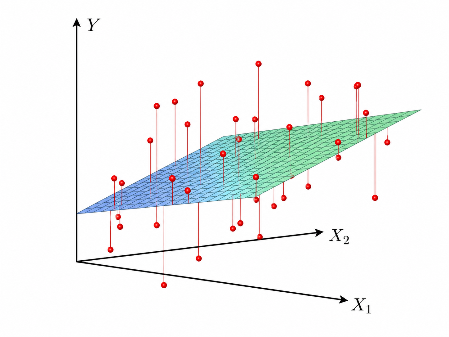
The analogue of a line in $2$ dimensions is the plane, and in higher dimensions we call it a hyperplane. We thus can use linear regression when we hypothesize that the data follows approximately a plane, as shown in the picture for the case when $d=2$.

No description has been provided for this image

The equation of a hyperplane is

$$ y = b + w_1 x_1 + \ldots w_d x_d \, , $$

where $b$ is sometimes called the intercept and the vector of parameters $w = [w_1, \ldots, w_d]$ control the slope. If we also let $x = [x_1,\ldots,x_d]$ be the vector for a point, the equation looks almost like the 1-d case:

$$ y = b + x\cdot w^T \, . $$

We can then provide the update rules for all the weights of the hyperplane model:

$$ w_i \leftarrow w_i - \rho \sum_{j=1}^n \left( \hat{y}_j - y_j\right ) X_{j,i} $$ and $$ b \leftarrow b - \rho \sum_{j=1}^n \left( \hat{y}_j - y_j\right ) . $$ Keep in mind that each update rule uses only the $i$-th coordinate $X_{j,i}$ from each of the input vectors $X_j$ in our data matrix $X$.

Here is a video of how a plane moves when its weights are changed with gradient descent in a number of iterations.

3.7 The Gradient Descent Algorithm: Efficiency and Implementation Issues ⬤ ¶

We now give simple pseudocode for the gradient descent algorithm. As discussed in the theory above, one update requires a computation that looks into the error of all points in our dataset. We will call this 'pass' over the entire dataset an epoch.

The following algorithm takes the number of epochs as a hyperparameter ($\mathit{nepochs}$). Implicitly, it also takes as a hyperparameter the overall algorithm of Gradient Descent, because - as we said - there are other ways to do the fit.

function w = LinearRegression-Fit ($X$,$y$)
Randomly initialize a $d$-dimensional vector $w$ and a scalar $b$
for $e=1$ to $\mathit{nepochs}$:
$g_0 = \sum_{j=1}^n \left( b + X_j w^T - y_j\right ) $
for $i=1$ to $d$:
$g_i = \sum_{j=1}^n \left( b + X_j w^T - y_j\right ) X_{j,i}$
$b = b - \rho \cdot g_0 $
for $i=1$ to $d$:
$w_i = w_i - \rho \cdot g_i$
return $w,b$

The algorithm returns the vector of parameters $w$ and $b$, that completely determine the model. Given that, inference (i.e. prediction) can be done with the following code.

function w = LinearRegression-Predict ($w,b,x$)
return $b+xw^T$

Looking at the algorithm we can observe at least two issues:

The vector $w$ is initialized randomly. However, we would like to be able to replicate experiments. Fortunately, there is a way to re-generate the same (pseudo)-random numbers, in the same order, and that is controlled via a hyperparameter that is called random_state in scikit-learn, and it appears in most algorithms that rely on randomness.
The algorithm needs to wait for an entire epoch before it does an update. This is a significant efficiency issue, especially when the dataset is big. It is also unnatural from a human learning point of view, as our intuition is that we learn with each and every error that we make.

3.7.1 Stochastic Batch Gradient Descent¶

Towards improving efficiency, we observe that a small sample of the points in $X$ would still follow the same hyperplane. We can thus use them as a proxy for the entire dataset. Ideally, we would want to use all training points. This gives rise to a randomized (or stochastic) variant of gradient descent. The main idea is to split the training set $X$ randomly into $n/k$ batches, each of size $k$ (here we assume that $k$ divides $n$), and perform one update for each batch, using exactly the same update rule as in gradient descent, but only using points from that batch. This leads to the following code:

function w = LinearRegression-Stochastic-Fit ($X$,$y$)
Randomly initialize a $d$-dimensional vector $w$ and a scalar $b$
Shuffle the rows (data points) of $X$
for $e=1$ to $\mathit{nepochs}$:
for $t=1$ to $n/k$:
$g_0 = \sum_{j=(t-1)k+1}^{t k} \left( b + X_j w^T - y_j\right ) $
for $i=1$ to $d$:
$g_i = \sum_{j=(t-1)k+1}^{t k} \left( b + X_j w^T - y_j\right ) X_{j,i}$
$b = b - \rho \cdot g_0 $
for $i=1$ to $d$:
$w_i = w_i - \rho \cdot g_i$
return $w,b$

In the extreme case when $k=1$ the algorithm is known as stochastic gradient descent. The batch size $k$ is a hyperparameter, because the output will be different for different values of $k$, even when the initialization is identical.

Batch gradient descent is in practice slightly slower per epoch, relative to ordinary gradient descent, but it may require a smaller number of epochs.

3.7.2 Scaling Features for Faster Learning¶

The total computational work for training a model is proportional to the number of epochs, so a faster learning per epoch is desirable. Scaling is a standard procedure for pre-processing data that can result in faster learning. The steps are the following:

For each attribute $i$, calculate the average $$\mu_i = \frac{1}{n}\sum_{j=1}^n X_{j,i}\,.$$
For each attribute $i$, calculate the standard deviation $$\sigma_i = \sqrt {\frac{1}{n}\sum_{j=1}^n (X_{j,i} -\mu_i)^2}\,.$$
For each point $j$ and attribute $i$, compute a new attribute $$ X'_{j,i} = \frac{X_{j,i}-\mu_i}{\sigma_i}\,.$$

In general, scaling features has the effect of bringing their spreads of values into balance, thereby changing the 'landscape' of the error function and perhaps making it more amenable to gradient descent methods.

3.8 Evaluating a Regression Model: Coefficient of Determination ⬤ ¶

Suppose now that after some epochs of training we have a regression model $y = f(X)$, after minimizing the total squared error

$$\mathit{SE}_{\mathit{model}} = \sum_j (y_j - f(X_j))^2 .$$

But how can we evaluate this model? Is the SE enough to evaluate its quality? The answer is no: if we just scale up all numbers by a factor of, say, 2, the SE will go up by a factor of 4, yet the model will be identical. We thus need a measure that is scale invariant.

For every regression problem we can construct a simple baseline model that simply always returns the average of the numerical labels of the training points. That is: $f(x) = \mathit{mean}\,(y)$. The total square error of this baseline model is then equal to:

$$ \mathit{SE}_{\mathit{base}} = \sum_j (y_j - \mathit{mean}\,(y))^2 . $$

We then define the coefficient of determination as:

$$ R^2 = 1 - \frac{\mathit{SE}_{\mathit{model}}}{\mathit{SE}_{\mathit{base}}}\, . $$

$R^2$ can be as high as 1, when the squared error is 0, and it will be 0 if our model is identical to the baseline model. In other words, we can always make sure that $R^2$ will be at least 0, although it could be even negative if our model is worse than the baseline.

3.9 RANSAC: Random Sample Consensus for Outliers ⬤ ¶

The existence of outliers can 'fool' a regression model, as illustrated in the following picture. There are many ways of handling outliers and their detection is a continuous research topic.

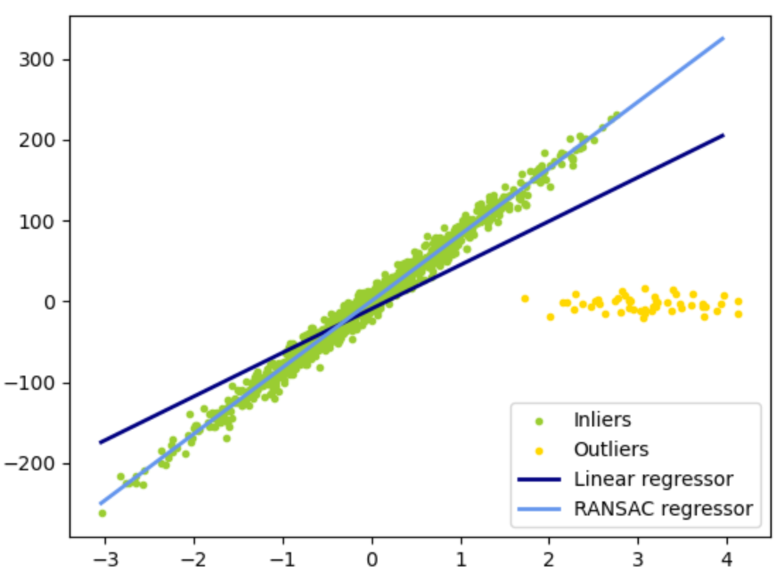
RANSAC is a simple but effective method for treating outliers. Here are its steps:

Hyperparameters:
$n'$: number of sampled points
$\theta$: inlier loss threshold
$n''$: inlier number threshold

Randomly sample $n'$ points $(X',y')$ from the data set $(X,y)$.
Fit a model $f$ to $(X',y')$.
Evaluate all points in $(X,y)$ with $f$ and keep only those that give a loss less than a threshold $\theta$. These are called inliers.
If the number of inliers is greater than $n''$, the model is good.
If the model is good, then return a new model fit on the inliers.

3.10 Feature Engineering ⬤ ¶

Fitting hyperplanes to data seems to have very limited power. However, transforming the data may render them explainable by linear models, i.e. make them amenable to linear regression. The transformation can be as simple as adding features to the data points, and working with engineered data sets that 'live' in higher dimensions.

As an example, consider the following picture.

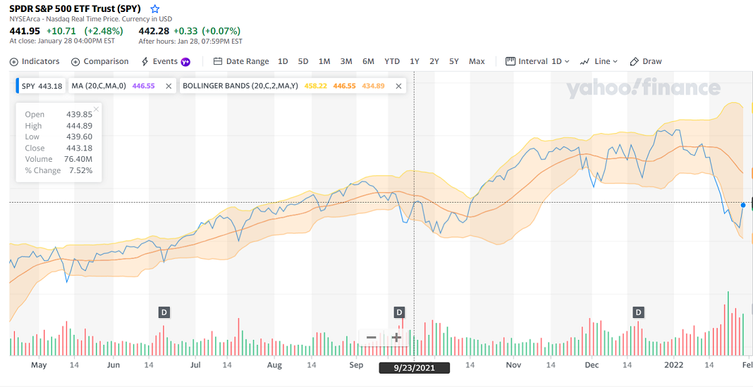
The blue line is the daily price of the S&P stock index, and the orange line is the average over the previous 20 days, which is a linear function of the 20 previous points. The upper and lower orange lines are computed by adding and subtracting the standard deviation of the values of the 20 previous points. Standard deviation involves calculations with the squares of the values, so these upper and lower bands are quadratic features, and a visual inspection can reveal that adding these features may be informative in making investment decisions.

3.11 Polynomial Regression ⬤ ¶

While engineering new features is limited only by our imagination, there are nevertheless some standard methods for constructing them. These are based on well-studied families of functions and their ability to fit data.

Quadratic Regression: Here we describe an example of quadratic regression on a 3-dimensional dataset. Given a point

$$ x = [x_1, x_2, x_3] \, , $$

we add the quadratic features to get the following point

$$ \tilde{x} = [x_1, x_2, x_3, x_1^2, x_2^2, x_3^2, x_1x_2, x_1x_3, x_2x_3] \, . $$

The 6 additional features are all the monomials of the polynomial $(x_1+x_2+x_3)^2$, when we expand it out.

Then the goal of quadratic regression is to find an 9-dimensional vector of weights $w$ (slopes), and the intercept $b$, and to construct a model with an equation of the form

$$ y = b + \tilde{x} \cdot w^T \, . $$

In other words, quadratic regression is identical to linear regression with the additional engineered features.

The exact same logic can be applied to cubic features, or features of any degree, and other non-linear functions. Of course, adding features comes at a computational cost.

3.12 Regression Code Notebook ⬤ ¶

Here is the code notebook.