Module 4 — Perceptron and Linear Separability
4.1 A Biological Neuron ⬤ 
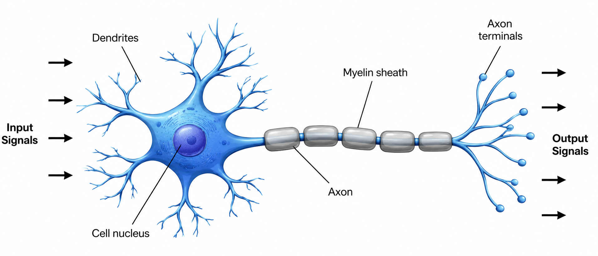
Biologists have studied animal neurons. A typical neuron works by taking a number of inputs that are chemical/electrical signals from other neurons through its dendrites. Not all incoming signals have the same 'weight': the brain is plastic and the dendrites modulate the signals before they are combined in the cell nucleus. When the combined modulated signals exceed some threshold (which may be different for each neuron), the neuron becomes activated and sends a signal to its output. Otherwise, the neuron is not activated.
Since the neuron appears to have two fundamental states (activated or not), we can speculate that it may be able to make binary decisions or classifications. This leads us to the mathematical modeling of a biological neuron as a perceptron.
4.2 Perceptron ⬤ 
We assume that the neuron/perceptron has $d$ inputs $x=[x_1,\ldots,x_d]$ and each input is modulated, i.e. multiplied by a corresponding weight $w = [w_1,\ldots,w_d]$. Thus what we call the net input is given by the following equation:
$$ z = wx^T = \sum_{j=1}^d w_j x_j\, . $$
The neuron then has an activation function $\phi(z)$ defined as follows for some activation threshold $\theta\,$:
- $\phi(z) =1$, if $z\geq \theta\:$ or $\:\phi(z) = 0$, if $z<\theta$ .
Another way to state the above rule is to set $b = -\theta$ and write it as follows:
- $\phi(z) =1$, if $wx^T + b\geq 0\:$ or $\:\phi(z) = 0$, if $wx^T+b< 0$ .
Some additional notation. For conciseness, we can set $w_0=b$ and let $w = [w_0,w_1,\ldots,w_d]$. Then, we can assume that all our points have an extra 'fixed' coordinate and they look like this: $x=[1,x_1,\ldots, x_d]$. In that case the rule becomes:
- $\phi(z) =1$, if $wx^T \geq 0\:$ or $\:\phi(z) = 0$, if $wx^T< 0$ .
4.3 Linear Separability ⬤ 
It is very useful to think about the points $x$ at which the perceptron is undecided, i.e. on the fence between the two decisions. Working with the definition, these are exactly the set of points $x$ that satisfy
$$ wx^T+ b =0\, .$$
This decision boundary, or decision surface, is the equation of a $d$-dimensional hyperplane, and the two decision regions will be what we call half-spaces.
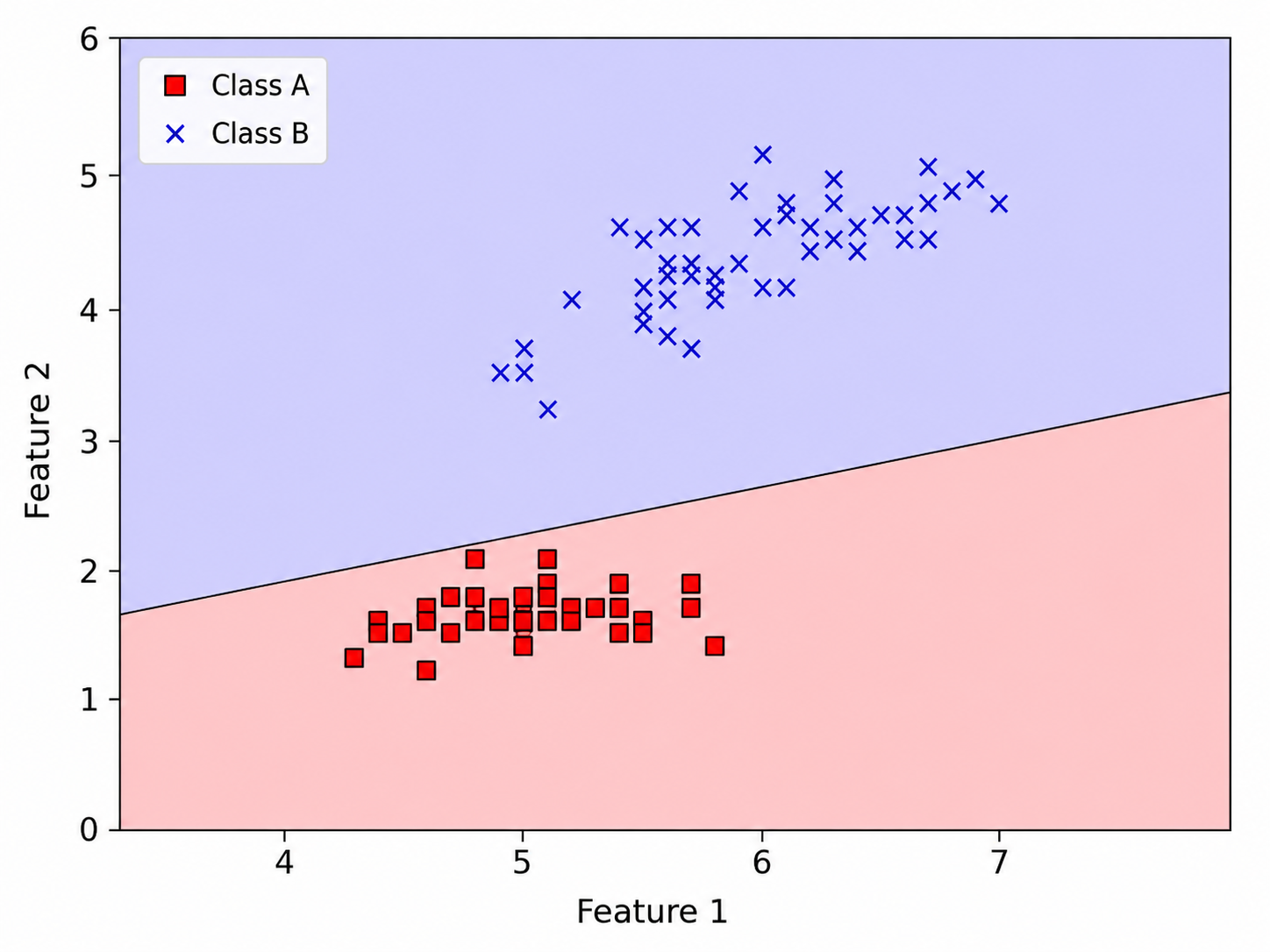
For a 2D example, the boundary is a line, while the two semi-planes are the two decision regions.
This leads us to the notion of linear separability: If we have a dataset $X$ where datapoints belong to two classes, and these two classes can be separated by a hyperplane, then we say that $X$ is linearly separable.
It follows, by definition, that if $X$ is linearly separable then there exists a perceptron that can separate it (and be 100% accurate on all points). And vice-versa, if $X$ is not linearly separable, then no perceptron can fully separate it.
4.4 The Perceptron Algorithm ⬤ 
We now want to come up with an algorithm that will learn the weights $w,b$ of a perceptron, so as to separate the classes of $X$ when $X$ is linearly separable. Recall that $X$ comes with a set of categorical labels $y$, and in this case we can set these labels to the numerical values $0$, $1$ so that they coincide with the possible outputs of the perceptron.
Here is the algorithm:
- function $w$ = Perceptron-fit ($X$,$y$)
- Randomly initialize a $d$-dimensional vector $w$ and a scalar $b$
- $\mathit{errorFlag} = \mathrm{True}$
- while $\mathit{errorFlag}$ do #new epoch starts here
- $\mathit{errorFlag} = \mathrm{False}$
- for $j=1$ to $n$:
- $z = b + X_j w^T$
- if $z\geq 0$ then $\hat{y} = 1$ else $\hat{y} = 0$ #in linear regression we use $\hat{y} = z$
- if $\hat{y} \neq y_j$ then $\mathit{errorFlag} = \mathrm{True}$
- $b = b - \left( \hat{y} - y_j\right ) $
- for $k=1$ to $d$:
- $w_k = w_k - \left( \hat{y} - y_j\right) X_{j,k} $
- return $w,b$
The algorithm strategy is to learn from each mistake. When the perceptron makes a mistake on a point $X_j$, then the weights $w,b$ are updated, and in fact the update rules are precisely the rules we used in stochastic gradient descent (with $\rho = 1$) for linear regression with one exception: $\hat{y}$ is now a categorical value $\{0,1\}$, whereas in linear regression we were using $\hat{y}=z$.
Like gradient descent, many variants of the perceptron algorithm are possible, with different learning rates $\rho$, stochastic variants and other variants involving batching, and so on. Note also that the algorithm can be run with other numerical values as class labels (such as $y,\hat{y}\in\{-1,1\}$).
The algorithm stops only when no $\mathit{errorFlag}$ is raised during an epoch, i.e. when all points are classified correctly. But is that guaranteed to happen?
Yes, as it turns out.
Fact 1: If $X$ is a linearly separable dataset, then the perceptron algorithm will eventually terminate.
There is an even stronger statement that can be made.
Fact 2: If $X$ is a linearly separable dataset, then one can compute a number $M$ that depends only on $X$, such that the perceptron algorithm will make at most $M$ mistakes during its course.
Fact 2 is known as the Rosenblatt-Novikoff Theorem. Frank Rosenblatt was the person that in 1958 came up with the idea of the perceptron, which according to many paved the way for modern Machine Learning [1]. You can find a proof and some other cool things about the perceptron in this link.
4.5 One-vs-One for Multilabel Classification ⬤ 
We now introduce the One-vs-One method for using perceptrons on multilabel data.
We will use a small example. Suppose that our data $X$ contains points with three labels: dog, cat, human. With this labeling, we can think of $X$ being partitioned into 3 submatrices: $X_{\mathit{cat}}$, $X_{\mathit{dog}}$, $X_{\mathit{human}}$. For each pair of data classes, we can train a perceptron. More specifically, we train the following classifiers:
- $C_1$, the cat-vs-dog classifier, using only data in $X_{\mathit{cat}}$ and $X_{\mathit{dog}}$.
- $C_2$, the human-vs-dog classifier, using only data in $X_{\mathit{human}}$ and $X_{\mathit{dog}}$.
- $C_3$, the human-vs-cat classifier, using only data in $X_{\mathit{human}}$ and $X_{\mathit{cat}}$.
Then, if we want to predict the label of a new point $x$, we first generate three different predictions from the classifiers $C_1$, $C_2$, $C_3$. Then we imagine a 'voting' process where each classifier votes for dog, human, or cat. The prediction that takes the most votes is the final prediction for $x$. If we have a tie, then we break it arbitrarily between the winners.
More generally, if we have data classes then we need to train ${k \choose 2} = k(k-1)/2$ different classifiers and use the majority rule.
4.6 Learning Logical Gates ⬤ 
Computer hardware and CPUs in particular, consist of millions of simple transistors implementing three basic logical functions: AND, OR and NOT.
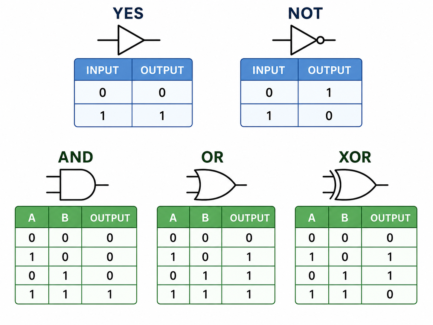
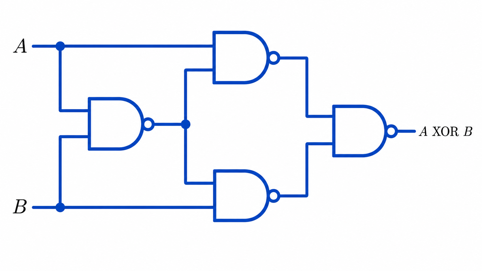
All other logical functions can be impemented using networks of these three basic gates. For example the XOR function (whose truth table is above) can be implemented as a 3-layer network of NOT-AND gates as shown here:
One way to see these logical functions (say the AND gate) is as a binary classifier that separates 4 points into two classes. Then one can ask this question: Can a perceptron 'learn' the 2-input OR gate? We can instantly see that the answer is yes by looking at the linear separability in the picture. Similarly, AND & NOT-AND are linearly separable.
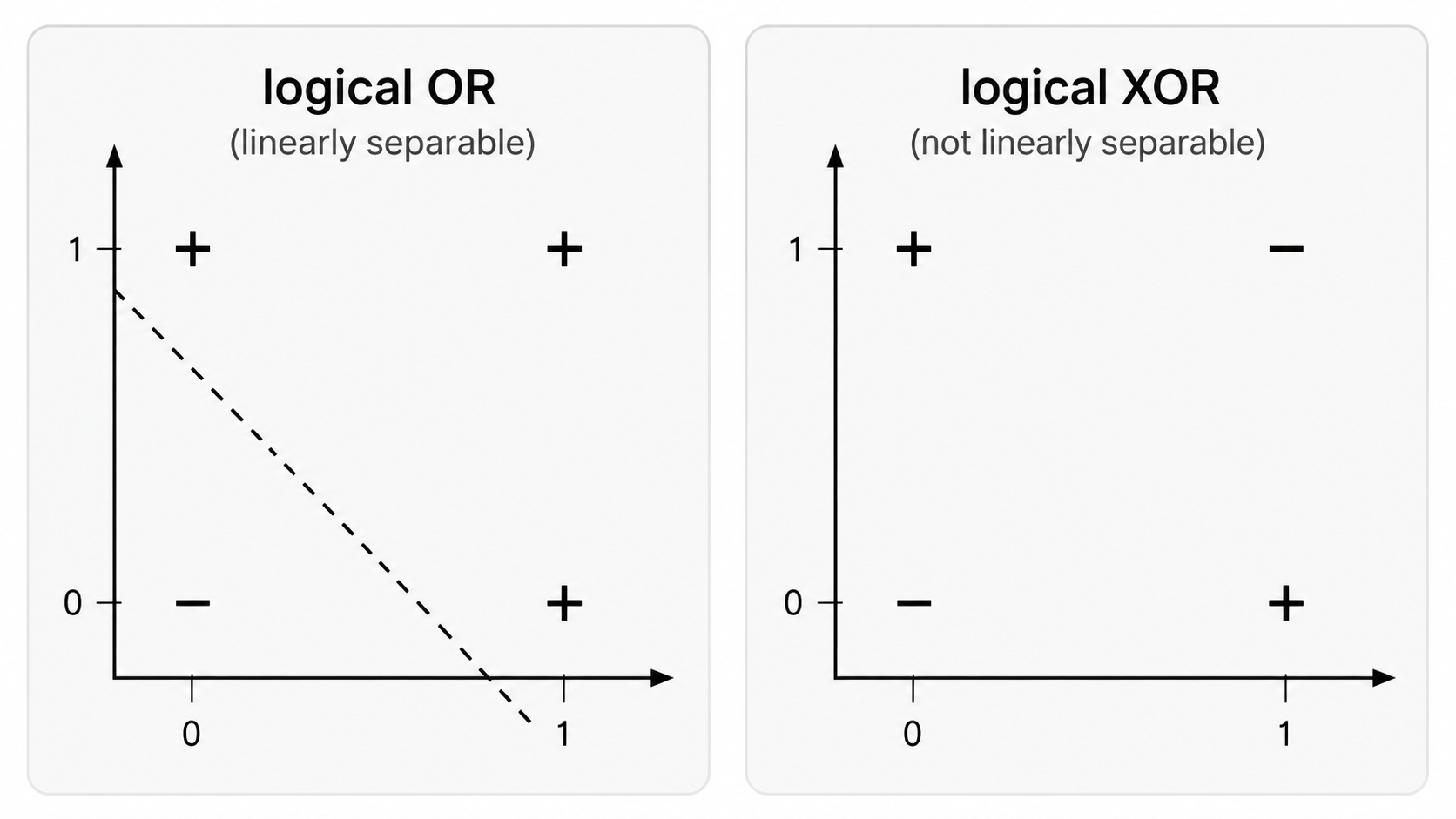
On the other hand, the XOR logical gate cannot be learned by a simple perceptron, but as we will see we a network of perceptrons can 'learn' the XOR gate.
Similarly to logical circuits in computers , it is believed that the high-level functionality of our brain emerges through networks of neurons. But what type of computational tasks can individual neurons perform? It was until recently believed that individual human neurons can only behave like simple separable logical gates, but there is now evidence that single neurons can actually be more complex and operate even like XOR gates [2].
4.6 Perceptron Code Notebook ⬤ 
Here is the code notebook.
4.7 Feature Engineering Revisited ⬤ 
Consider the picture on the left. The dataset is clearly not separable, so it can not be learned by a perceptron.
To each point $(x,y)$ in our dataset, we now add one extra feature/coordinate, $x^2+y^2$, so that the point becomes $(x,y,x^2+y^2)$.
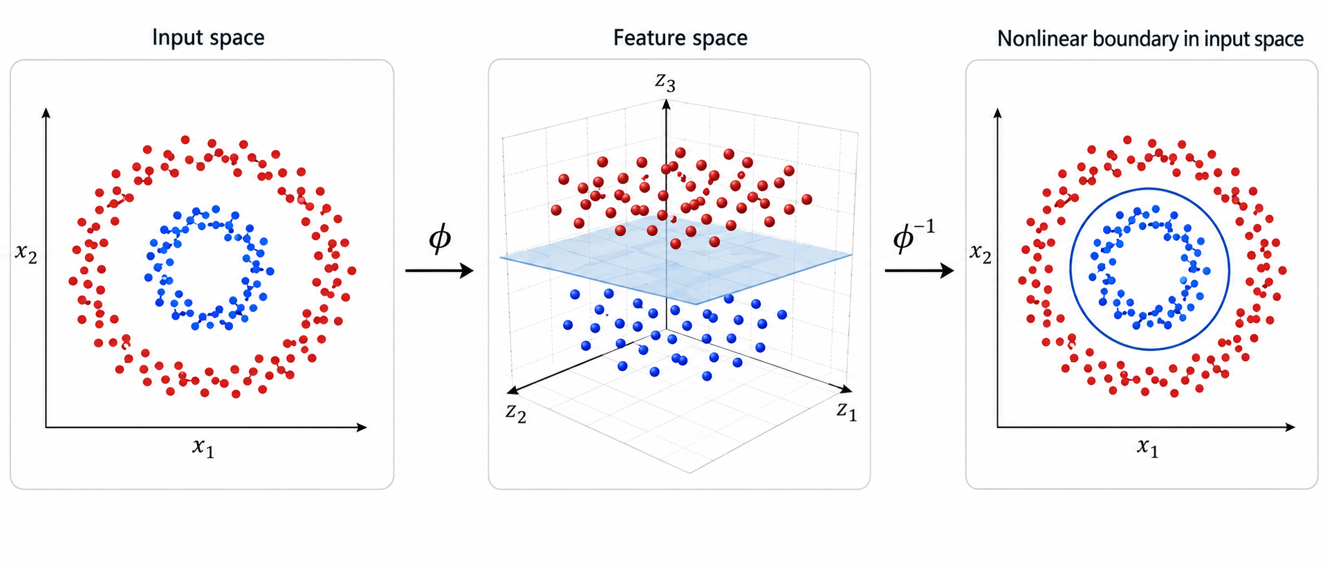
This 'engineered' 3D-dataset is plotted in the second figure. We can see that the dataset has now become linearly separable. Specifically we see that the plane separating the two classes is defined by $x^2+y^2 = 0.5$; that is, the third coordinate is equal to 0.5. If we go back to the original space, the set of points $(x,y)$ that satisfy the equation $x^2+y^2 = 0.5$ is a circle of radius $1/\sqrt{2}$. The linear separation surface in 3D becomes a non-linear surface in 2D.
This is yet another example of the power of feature engineering. However, generally speaking, engineering appropriate features is a difficult task that requires a very good understanding of the application and/or the dataset.
4.8 Perceptron Weaknesses ⬤ 
We can now identify some weaknesses of the perceptron:
- Given a linearly separable dataset $X$, the number of perceptrons that can separate the classes is usually infinite. The output of the perceptron learning algorithm depends on the random initialization and the order in which the points are visited by the algorithm.
- In some cases, the algorithm can learn a perceptron with a decision surface that is much closer to one of the classes than it is to the other. That is demonstrated in the following figure. Intuitively speaking, such decision surfaces are undesirable since we should not have any a priori preference for any class.
