Module 5 — Logistic Regression
5.1 The Logistic Neuron ⬤ 
Thinking of a biological neuron as having just two (1/0) states of excitation is an oversimplification. The neuron does have a continuous range of outputs with a very sharp transition from 0 to 1, around the threshold. That leads us to the definition of the logistic neuron shown (in the case of 2D) in the following picture.
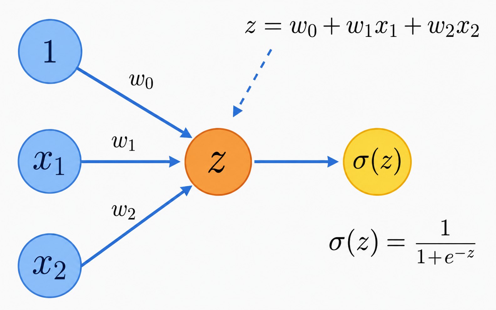
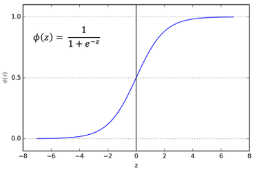
The activation of the logistic neuron is the sigmoid function
$$ \sigma(z) = \frac{1}{1+\exp\,(-z)} \, , $$
which does have a steep transition around $z=0$.
We can convert this activation into a binary classification decision as follows:
- if $\sigma(z)\geq 0.5$, then the classification output is 1.
- if $\sigma(z)<0.5$, then the classification output is 0.
Comment: We can use any other threshold (not just 0.5) for converting the activation into a decision, and that choice may depend on the application. In these notes, we will stick with the standard choice, 0.5.
5.2 Properties of the Logistic Neuron ⬤ 
We can start by asking whether the sigmoid function enables us to learn non-linear classification surfaces. Looking at the behavior of the sigmoid function, we see that it is monotonically increasing. The points $x$ that are exactly on the class boundary give a net input of $z=0$, i.e. they satisfy $$ wx^T + b = 0 \, . $$
This is again the equation of a hyperplane, and so the logistic neuron is a linear classifier. However, its ability to output a continuous range of values offers some concrete advantages.
- We can interpret the output as a probability that the input point is in class 1.
- Because the probabilities are continuous within the range $[0,1]$, we can define a measure of error for each prediction. We can then generalize to an overall error or loss over the entire dataset, and seek to find the parameters that minimize it, as we did in the case of linear regression. This task is referred to as logistic regression.
5.2.1 Sigmoid Activation: a Justification
Suppose an event happens with probability $p$. We can then define the odds ratio of the event (a quantity that is commonly used for betting) as: $$ \mathit{odds}\,(p) = \frac{p}{1-p}\, . $$
The odds are a positive number, but we can convert it to a real number in the range $(-\infty,\infty)$ by using the logit function
$$ \mathit{logit}\,(p) = \log\left(\frac{p}{1-p}\right) $$
If we now interpret the net input $z$ as the logit function of an event, i.e. if we set $$ z= \log\left(\frac{p}{1-p}\right) \, , $$ solving for $p$ gives us $$ p = \frac{1}{1+e^{-z}} \, . $$
Thus, the sigmoid function can be viewed as a probability if we view the net input as the logit function of an event.
5.3 Loss Function ⬤ 
5.3.1 Likelihood: A Measure of Goodness
Suppose we evaluate a point $X_j$ with a logistic neuron, and we get a probability $\hat{y}_j$. Imagine for a moment that the logistic neuron does not output $1$ or $0$ based on whether $\hat{y}_j$ is greater than the threshold, but instead outputs $1$ with probability $\hat{y}_j$ and $0$ with probability $1 - \hat{y}_j$. Then the probability that the neuron's output is correct is as follows (where $y_j$ is the true label):
$$ p_j = \left\{ \begin{array}{cl} \hat{y}_j & \mathrm{~~if~~} y_j = 1 \, , \\ 1-\hat{y}_j & \mathrm{~~if~~} y_j = 0 \, . \end{array} \right. $$
The probability that the neuron outputs the correct answer for $X_j$ is called the likelihood of that point. Often it is convenient to write the likelihood in the form of a single equation:
$$ p_j = \hat{y}_j^{y_j} {(1-\hat{y}_j)}^{(1-y_j)} \, . $$
When we have $n$ points, we can then calculate their overall likelihood, by multiplying the individual likelihoods:
$$ P(w,b|\,X) = \prod_{j=1}^n p_j \, . $$
Here we write $P(w,b|\,X)$ to emphasize that this likelihood depends only on the values of the parameters $w,b$ of the logistic neuron, for the case where the neuron is applied to data set $X$. We want then to pick parameters $w,b$ that maximize the overall likelihood. When it is clear that we are talking about set $X$, we can simply write the likelihood as $P(w,b)$.
5.3.2 The Negative Log-Likelihood Loss
To make things consistent with our approach to linear regression, instead of maximizing the likelihood we can equivalently minimize the negative log-likelihood loss function:
$$ L(w,b) = - \log_2 P(w,b) = - \log_2 \prod_{j=1}^n p_j = - \sum_{j=1}^n \log_2 p_j = \sum_{j=1}^n l_j \, , $$ where $$ l_j = -\log_2 p_j = -y_j \log_2 \hat{y}_j - (1-y_j) \log_2 (1-\hat{y}_j) \, . $$
This has the additional nice property that the loss has become additive over the data points, in that each data point $X_j$ contributes its own individual negative log-likelihood loss $l_j$.
Comment: It is worth taking an extra look at $l_j$. Consider the case when $\hat{y}_j=1$. The loss $-\log_2 \hat{y}_j$ can be viewed as a measure of the 'surprise' we get when we predict probability $\hat{y}_j$. Or, in some sense, it can be viewed as a measure of how much information we gain from that specific point, about the quality of our classifier. Measuring information as the log of some probability has its root in information theory. Indeed $l_j$ bears some similarity with the entropy function, but because it involves two probability distributions, $[\hat{y}_j,1-\hat{y}_j]$ and $[y_j,1-y_j]$, it is actually related to the cross-entropy function. The notions of entropy and cross-entropy came out of an MS thesis written by Claude Shannon [1].
5.4 Stochastic Batch Gradient Descent for Logistic Regression ⬤ 
The algorithm is this:
- function w = LogisticRegression-Stochastic-Fit($X$,$y$)
- Randomly initialize a $d$-dimensional vector $w$ and a scalar $b$
- Shuffle the rows (data points) of $X$
- for $e=1$ to $\mathit{nepochs}$:
- for $t=1$ to $n/k$:
- $g_0 = \sum_{j=(t-1)k+1}^{t k} \left( \sigma(b + X_j w^T) - y_j\right ) $
- for $i=1$ to $d$:
- $g_i = \sum_{j=(t-1)k+1}^{t k} \left( \sigma(b + X_j w^T) - y_j\right ) X_{j,i}$
- $b = b - \rho \cdot g_0 $
- for $i=1$ to $d$:
- $w_i = w_i - \rho \cdot g_i$
- return $w,b$
This is precisely the same algorithm we saw for linear regression. There is only one small difference: we now use the function $\sigma(b + X_j w^T)$ instead of $b + X_j w^T$ in the update rules. The difference seems superficial because $\sigma(b + X_j w^T)$ is the output of the logistic neuron, and $b + X_j w^T$ is the output of the linear regression model.
However, it is NOT correct to assume that the model outputs always appear in gradient descent update rules for other learning algorithms: these update rules are derived using the gradient of the loss function associated with the learning algorithm! For logistic regression, the loss function is the negative log-likelihood. Can you compute its gradient?
5.5 One-vs-Rest Classification ⬤ 
The fact that logistic neurons output a probability is used in the one-vs-rest method for multilabel classification.
Consider for example a dataset $X$ with three labels: cat, dog, human. We can then consider $X$ as consisting of three sets of points $X_{\mathit{cat}}$, $X_{\mathit{dog}}$, $X_{\mathit{human}}$. We will train three different binary classifiers:
- One where points in $X_{\mathit{cat}}$ have label 1 and the combined points $X_{\mathit{dog}}, X_{\mathit{human}}$ have label 0.
- One where points in $X_{\mathit{dog}}$ have label 1 and the combined points $X_{\mathit{cat}}, X_{\mathit{human}}$ have label 0.
- One where points in $X_{\mathit{human}}$ have label 1 and the combined points $X_{\mathit{cat}}, X_{\mathit{dog}}$ have label 0.
Given the trained classifiers and a point $x$, each of these three classifiers outputs a probability for $x$: $p_{\mathit{cat}}$, $p_{\mathit{dog}}$, and $p_{\mathit{human}}$. We can then assign $x$ to the class that gets the highest probability. For example, if $p_{\mathit{dog}}>p_{\mathit{cat}}$ and $p_{\mathit{dog}}>p_{\mathit{human}}$, we can output the classification dog for $x$. In the unlikely case we have a tie, we can resolve it arbitrarily.
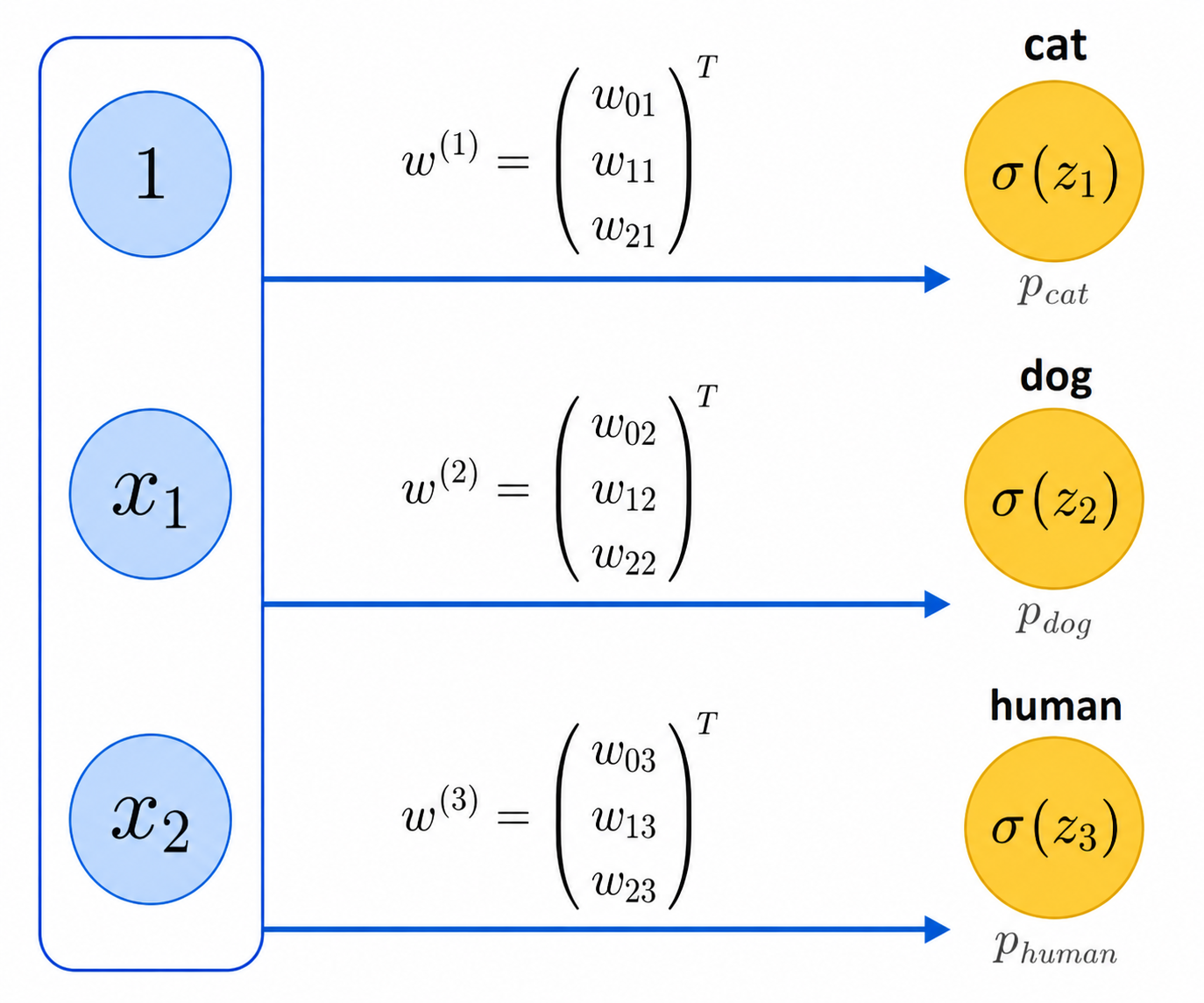
We can think of these 3 classifiers as a 2-layered 'network' of neurons (as shown in the figure above), although the network is still trivial since the 3 neurons do not interact with each other.
More generally, if we have $k$ labels, we will train exactly $k$ one-vs-rest classifiers. The number of trained classifiers is much smaller than the $k(k-1)/2$ classifiers required by the one-vs-one method. However, we should observe that we now train these $k$ classifiers on the entire dataset $X$. Thus, training one such classifier is going to be more expensive relative to training a single classifier in the one-vs-one method. Overall, one-vs-one will likely be faster to train, for most datasets $X$.
Comment: The $k$ probabilities $p_1,\ldots, p_k$ returned by the $k$ classifiers will very likely not sum up to 1. We can however 'normalize' them into a probability distribution, by returning the probabilities $$p_j' = \frac{p_j}{\sum_{i=1}^n p_i}$$ for each $j=1,\ldots,k$. The scikit-learn one-vs-rest implementation outputs such normalized probabilities.
5.6 Logistic Regression Code Notebook ⬤ 
Here is the code notebook .