Module 6 — Regularization
6.1 Sensitivity to Noise ⬤ 
Consider as a visual example the following 2D dataset.
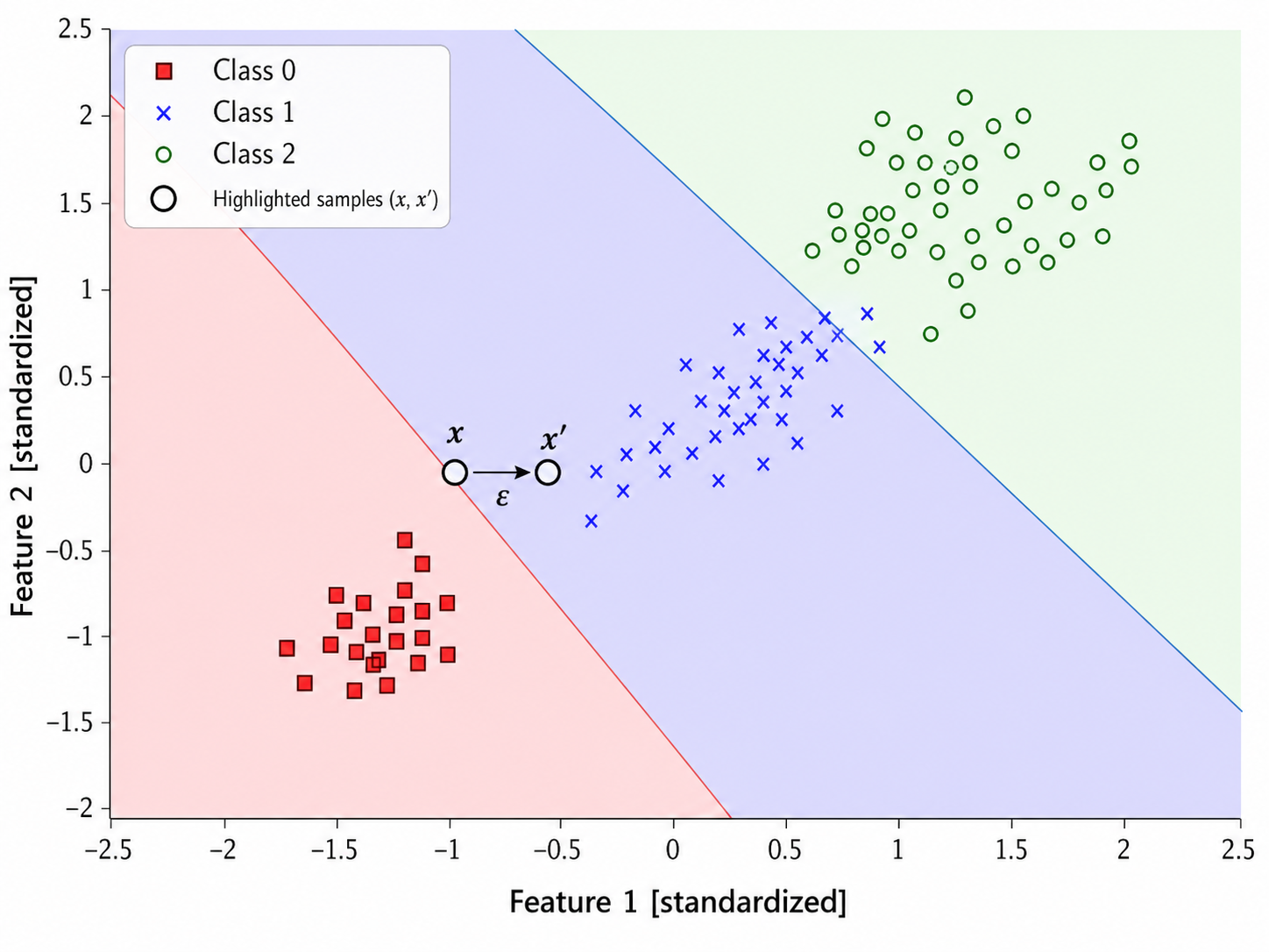
Suppose now we have one point $x=(x_1,x_2)$, and a second one $x' = (x_1+\epsilon,x_2)$, which comes from adding a bit of noise $\epsilon$ to $x_1$. Since we expect that nearby points in space should belong to the same class, the classifier should not be too sensitive to the noise.
Let's then consider the net input of a classifier with weights $[w_0,w_1,w_2]$ for our two points:
- $z = w_1 x_1 + w_2 x_2 + w_0$, and
- $z' \: = \: w_1(x_1+\epsilon) + w_2x_2 + w_0 \: = \: z + w_1\epsilon$.
Intuitively, if $w_1$ is large, then even a small amount of noise $\epsilon$ will cause a large change in the net input $z$.
From this we can see that smaller values of the parameters $w_i$ would be preferred, since they may lead to better generalization. That leads us to regularization, a class of techniques meant to fight overfitting.
6.2 Regularization ⬤ 
We would like to impose a penalty to large values for the parameters $w$. This can be done by adding a penalty to the loss function. More specifically, if our loss function is $L$, we can then define a new loss function $$ L_{\mathit{reg}}(w) = L(w) + \lambda\,\|w\|_2^2 \, , $$ where $\lambda$ is some hyperparameter that controls the strength of regularization. This new loss function imposes a penalty to having a large 2-norm of the weights, which is the reason it is called $l_2$-regularization. Note that if $\lambda$ is large, the optimization favors those choices of $w$ for which $\|w\|_2$ is smaller, which in turn forces smaller values for the individual weights $w_i$. Also note that some applications may use the unsquared 2-norm, $$ L_{\mathit{reg}}(w) = L(w) + \lambda\,\|w\|_2 \, , $$ which penalizes the growth in vector norm linearly rather than quadratically. (With the learning algorithms covered in this course, the squared 2-norm is more commonly used.)
Alternatively, we can perform $l_1$-regularization by defining this loss function as $$ L_{\mathit{reg}}(w) = L(w) + \lambda\,\|w\|_1 \, . $$
Regularization can also be applied to linear regression, where $l_2$ and $l_1$ regularization are known as Ridge and Lasso regression, respectively. A mix of $l_2$ and $l_1$ regularization that adds two different regularization terms is known as elastic nets.
These new loss functions penalize for large weights and intuitively will make it harder for the line to be 'dragged' by one outlier; hence, the model will be less prone to overfitting. These loss functions can be optimized with an appropriate optimizer. Usually a standard optimizer can treat (via gradient descent) the $l_2$ regularization without any difficulties, but optimizing with $l_1$-regularization is a harder computational problem.
6.3 Geometric Understanding of Regularization ⬤ 

Consider the pictured landscape of a loss function of a two dimensional model, where the $z$-axis is the value of the loss. Pairs $(x,y)$ that give the same loss value $L$ are plotted with the same color at height $z=L$. These contours are called a level set of the function. Level sets form closed curves if we 'project' them onto the 2D plane.
Let's now consider the $l_2$-regularization loss function $L_{\mathit{reg}}(w) = L(w) + \lambda\,\|w\|_2^2$. This is a sum of two different functions: a loss (or 'cost') $L(w)$, and a penalty $\lambda\,\|w\|_2^2$. The following image shows the contour plots of both functions in a simple 2D example. The contour plot of the regularization part consists of circles, because the set of points that are on the same level $L$ define the circle $w_1^2+w_2^2=L$.
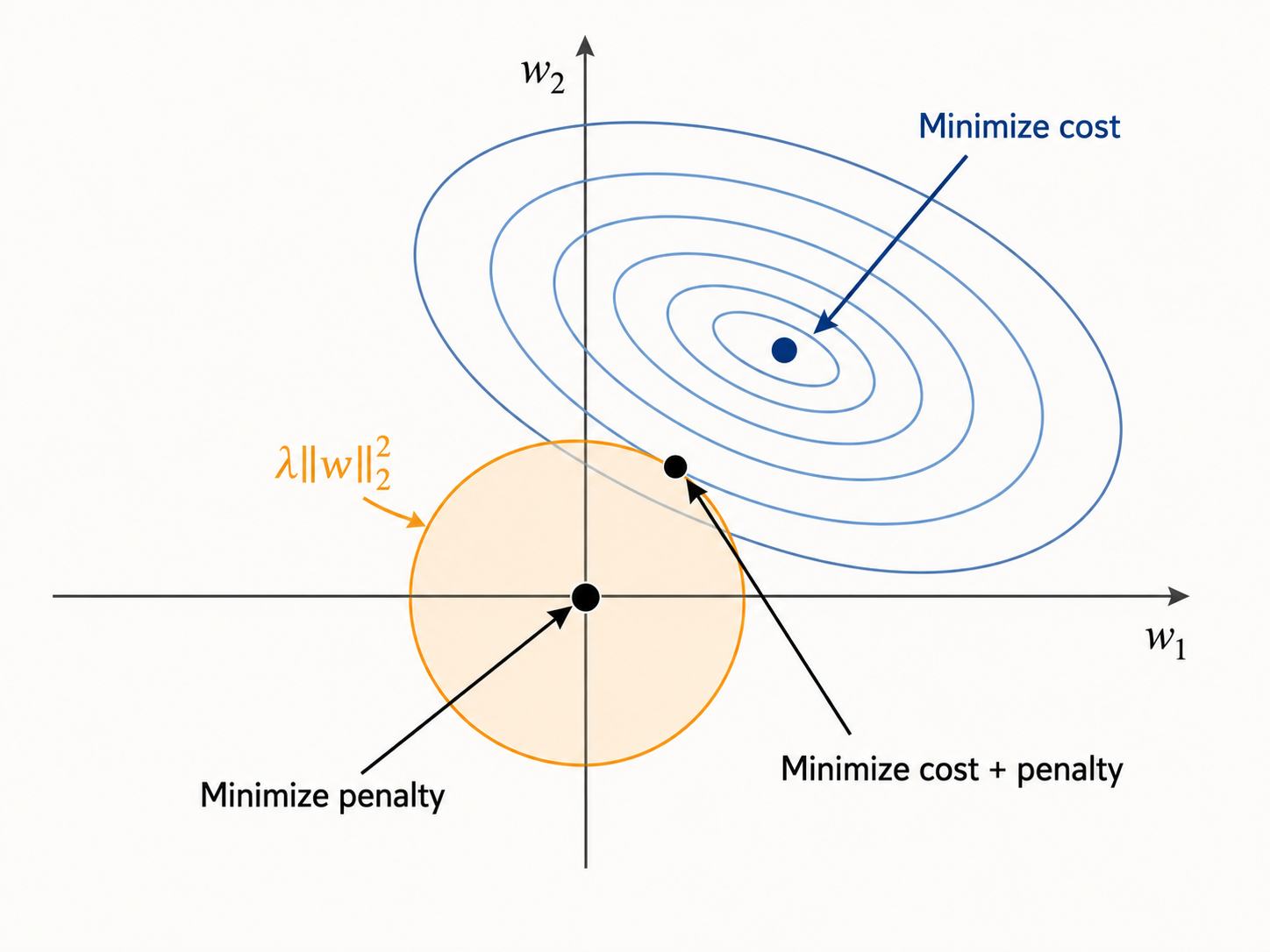
There are two different points that minimize each part separately, but their sum is minimized at a different intermediate point. In fact, in the case of $l_2$-regression, there is a unique tangent line to the corresponding contour curves of the two functions.
Now consider the $l_1$-loss regularization $L_{reg}(w) = L(w) + \lambda\,\|w\|_1$ and the corresponding contour plots.
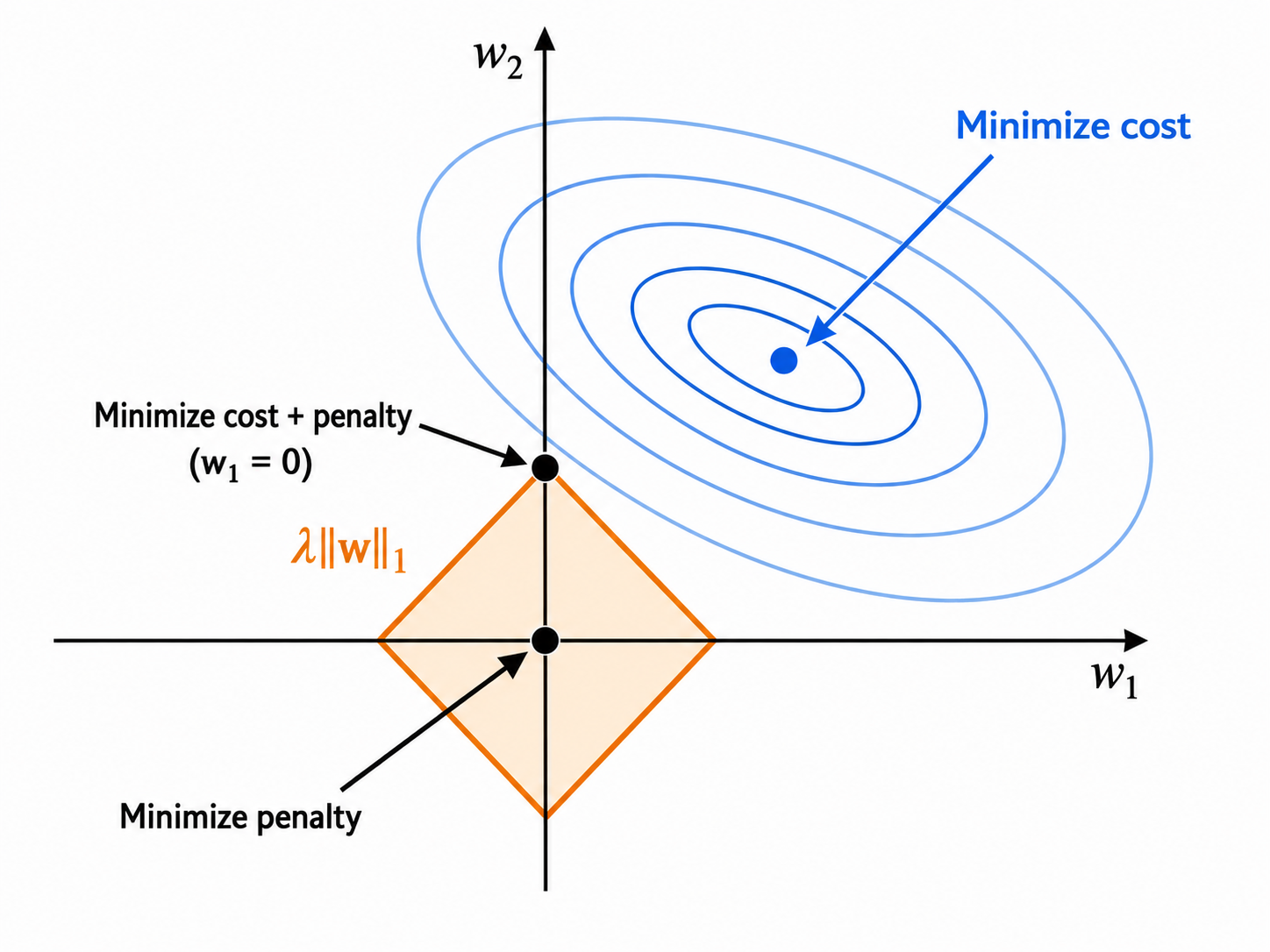
In this case, the contour plots of the regularization term are squares around the origin, since the equations $|w_1|+|w_2|=L$ define squares. Again, the sum of the two functions is minimized at an intermediate point.
$l_1$-regularization has a very interesting characteristic. Because the loss function $L(w)$ is convex, and $\|w\|_1$ has square-like contours, it is very likely that the corners of $\|w\|_1$ will penetrate deeper towards the center of the convex contours of the loss function. Intuitively, the sum of the two functions will be minimized at these corners of $\|w\|_1$ (even in higher dimensions), i.e. at points where many weights $w_j$ are equal to 0. In the picture we see that the minimium occurs at $w_1=0$.
Thus, whenever we do $l_1$ regularization the solution vector $w$ is likely to have multiple zero entries. This may imply that the corresponding inputs/attributes are not as important as the others (e.g. if $w_1=0$, then the feature value $x_1$ may not so relevant). Thus we can use $l_1$ regularization as a means of determining those features that are more 'relevant' or 'impactful'.