Module 7 — Support Vector Classifiers¶

7.1 The Inductive Bias of SVCs ⬤ ¶

margin as the inductive bias of SVCs

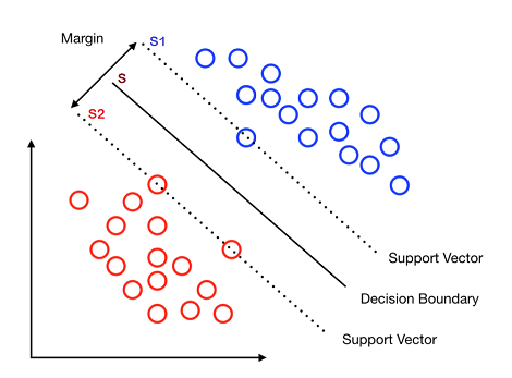
Given a hyperplane $S$ that linearly separates two classes of points, one can imagine all possible hyperplanes that are parallel to $S$. Among these two hyperplanes there exist exactly two hyperplanes $S_1,S_2$ that still separate the two classes, but just barely: at least one point from each class is exactly on the corresponding hyperplane. An illustration in the case of 2D data is given in the above picture.

Of course, given $S_1$ and $S_2$ it makes sense that the decision boundary $S$ should be set exactly half-way between the two. That is not necessarily the case with the perceptron, or logistic regression, but we can introduce it here as a meaningful learning (inductive) bias.

Now consider the distance between $S_1$ and $S_2$, which is what we call the margin. Notice that if we slightly tilt $S$ and get two different hyperplanes $S_1$ and $S_2$, then the margin will change. Then it would make sense to find the hyperplane $S$ that gives the largest possible margin, since that intuitively gives less room for future errors. We can then introduce margin maximization as an additional inductive bias. (Note that other definitions of margin have been used, particularly in theoretical proofs.)

The support vector machine (SVM) is a large margin classifier: it aims to find the decision boundary that maximizes the margin between the two classes. SVM gets its name from the fact that the margin depends only the boundary points, which are also called support vectors (because they are 'supporting' $S_1$ and $S_2$).

7.2 A Mini-Review of Basic Math ⬤ ¶

7.2.1 Parallel Hyperplanes and their Equations¶

Suppose that our decision hyperplane $S$ has the equation $wx^T + b = 0$. We can also assume that the blue class (which is farther from the origin) satisfies $wx^T + b \geq 0$.

Notice that for any constant $c\neq 0$, the hyperplanes $cwx^T + cb = 0$ and $wx^T + b = 0$ are the same; that is, uniformly scaling the parameters of $S$ does not change $S$. Then we can assume that the parameters are already appropriately scaled so that the blue support point $x_{\mathit{blue}}$ satisfies $wx_{\mathit{blue}}^T + b = 1$, which means that the equation for $S_1$ will be $$ wx^T + b - 1 = 0\, . $$

Since hyperplane $S_2$ is at the same distance from $S$, its equation will be $$ wx^T+b+1=0\, . $$.

7.2.2 Distance between Two Parallel Hyperplanes¶

Let $wx^T + b=0$ be the equation of a hyperplane $S$. Then the distance between the origin and the closest point in $S$ is equal to: $$ d = \frac{|b|}{\|w\|_2}\, . $$

We now have two support hyperplanes $S_1$ and $S_2$ with the following distances from the origin: $$ d_1 = \frac{|b-1|}{\|w\|_2} \mathrm{~~~~and~~~~} d_2 = \frac{|b+1|}{\|w\|_2} \, . $$

If we assume that $d_1>d_2$ (as in the figure above), it follows that $b<0$. In this case, we get that the distance between the two hyperplanes is:

$$ d = d_1-d_2 = \frac{2}{\|w\|_2} \, . $$

7.2.3 Inner (Dot) Product as a Similarity Measure¶

Given some row vector $x$ of dimensions $1\times d$, we can express its Euclidean norm as follows: $$ \|x\|_2^2 = x \cdot x^T \, . $$ This can be verified easily by calculating the dot product $x \cdot x^T$.

Consider now the Euclidean distance of two points $x_1$ and $x_2$. Using the above fact about dot products, we have: $$ \|x_1-x_2\|_2^2 = (x_1-x_2)(x_1 - x_2)^T = \|x_1\|_2^2 + \|x_2\|_2^2 - 2x_1x_2^T \, . $$

We see here that for two vectors $x_1$, $x_2$ that have some fixed norm, what really controls their Euclidean distance is their dot product $x_1x_2^T$. We can thus think of the dot product as a similarity measure (since an increase in $x_1 x_2$ results in a decrease in the distance $\|x_1-x_2\|_2$).
The dot product of two vectors is an example of an inner product.

We have seen how engineered features can be very powerful in combination with linear classifiers. Using kernels like $$K(x_1,x_2) = \exp\,(-\|x_1-x_2\|_2)$$ for measuring similarity can be shown to be equivalent to computing the inner product $\phi(x_1)\phi(x_2)^T$, where $\phi(x_1)$ and $\phi(x_2)$ are transformations of the original points. Such transformed vectors can have even an infinite number of 'engineered' features.

7.3 The Objective in SVCs ⬤ ¶

Let's consider again a 2D example in this picture:

SVC 2d example

The dataset $X$ consists of two sub-datasets, $X_{blue}$ and $X_{red}$. Our inductive bias requires that the following constraints are satisfied:

for each $x\in X_{blue}$, we have $xw^T + b -1 \geq 0$;
for each $x\in X_{red}$, we have $xw^T + b +1 \leq 0$.

This means that if we have a total of $n$ points, we have $n$ different inequalities that must be satisfied.

Given these constraints we then want to maximize the distance between the two hyperplanes, i.e. we want to maximize $2/\|w\|_2$. Equivalently we can minimize $$ \|w\|_2^2 = w^T w \, . $$

7.4 Optimization and the Kernel Trick ⬤ ¶

We have now to minimize a quadratic function $\|w\|_2^2$ under some linear constraints (i.e. linear inequalities). This is a case of a general class of problems that is called quadratic programming.

Algorithms for quadratic minimization problems are beyond the scope of this course. But an extremely interesting possibility is that instead of solving directly the above problem, we can instead solve the so-called 'dual', an equivalent problem where the quadratic term to be minimized is something of the form $\alpha^T Q \alpha$, where $\alpha$ is a set of parameters, and $Q$ is the matrix defined as follows:

$Q_{ij} = x_ix_j^T$ if points $x_i$ and $x_j$ have the same label;
$Q_{ij} = - x_ix_j^T$ otherwise.

In this case, the minimization algorithm relies only on the matrix $Q$, which involves pairwise similarities between our points and it really does not require knowing the individual points! Thus we can 'learn' a linear separating hyperplane $S$ by relying only on inner products.

However, as we discussed above, we can replace the inner-product notion of similarity (that comes from Euclidean distance), with other types of similarity measures. In that case, we will (essentially) be learning hyperplanes with transformed high-dimensional points, that can be then translated back to non-linear separation surfaces in the original space. However, these transformed high-dimensional points will never be explicitly calculated by the algorithm, because the algorithm does not require the points, but only their distances!

All this means that SVMs can be computed by essentially the same algorithm on such transformed data, by simply changing the notion of similarity. That is why SVM algorithms offer as a hyperparameter the choice of a kernel as the similarity measure.

This procedure has become known as the kernel trick. The following image is a common visualization of how linear separation in higher dimensions can be equivalent to nonlinear separation in the original space.

Visualization for kernel trick .

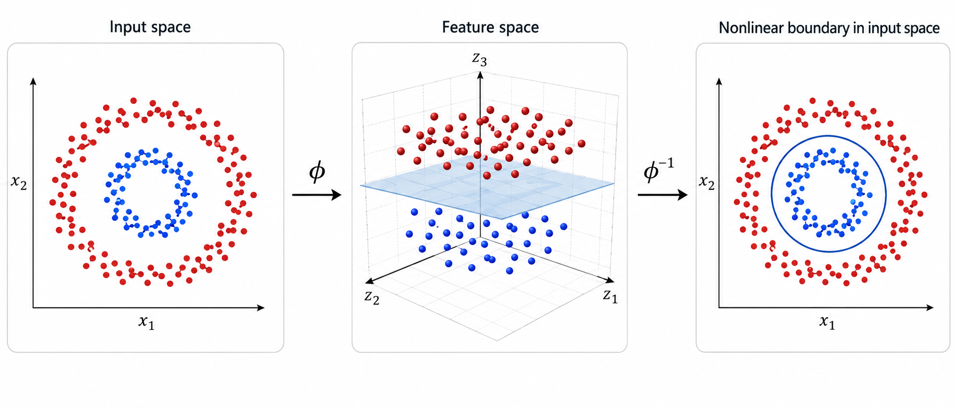The kernel trick is a very interesting way of performing nonlinear classification. However, the computational requirements of the algorithm are quite high, and as a result the algorithm can be used only in relatively small data sets.

7.5 Slacks: Regularization and Nonlinear Separability in SVCs ⬤ ¶

With the definition we have seen so far, SVCs are not equipped to learn data that is not linearly separable. The algorithm will simply fail to return any model.

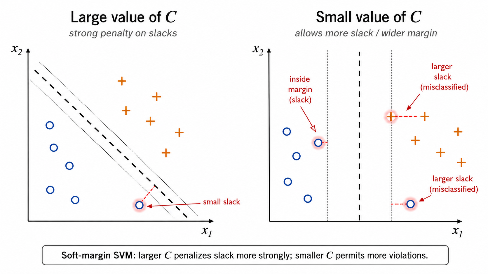
As with any machine learning algorithm, an SVM is also subject to overfitting. A single point can force the margin to be too small, as shown in the left-hand image. Forcing the SVM to correctly classify every point may result in an overly-complex decision boundary.

To address both the linear separability issue and the overfitting issue, we allow points to violate the strict inequalities for the surfaces $S_1$ and $S_2$. We do this by giving to each point $X_i$ a slack parameter. We do that by introducing an extra variable $\zeta_i$, with the constraint that $\zeta_i\geq 0$. We can then relax the strict inequalities to:

for each $X_i \in X_{\mathit{orange}}$, we have $X_iw^T + b -1 +\zeta_i \geq 0$.
for each $X_i \in X_{\mathit{blue}}$, we have $X_iw^T + b +1 - \zeta_i\leq 0$.

Of course, without any further constraints the slacks can take arbitrary values. So we have to impose an additional penalty for the total slack used by the points. That means that we now want to minimize $$ \min \|w\|_2^2 + C \sum_{i=1}^n \zeta_i \, . $$

Here $C$ is the inverse strength of regularization. If we let $C$ be very large, then minimization will have to make the slacks very small — that is, the slacks would not play a big role.

No description has been provided for this image

7.6 Optimization Again: The Hinge Loss ⬤ ¶

We can write the loss function as follows: $$ \min \|w\|_2^2 + C \sum_{i=1}^n \max\left\{0,1 - \mathrm{sign}(y_i-0.5)\,(X_iw^T +b)\right\}\, . $$

Notice that when $y_i=1$, we pay a penalty of $1- (X_iw^T+b)$ which is precisely equal to $\zeta_i$ (as defined for class 1). When $y_i=0$, the penalty is $1+ (X_iw^T+b)$ which is again equal to $\zeta_i$ (as defined for class 0).

Replacing the slacks with this so-called hinge loss allows the use of gradient descent for finding the best weights. Gradient descent is usually much faster than quadratic programming, but it is limited only to linear classification, since it cannot be made to work with the kernel trick. That is the reason scikit-learn has two different implementations of SVMs: sklearn.svm.SVC and sklearn.svm.LinearSVC.

7.7 SVM Code Notebook ⬤ ¶

Here is the code notebook for SVM.