Machine Learning Notes

Module 8 — Decision Trees

8.1 What Is a Decision Tree? ⬤

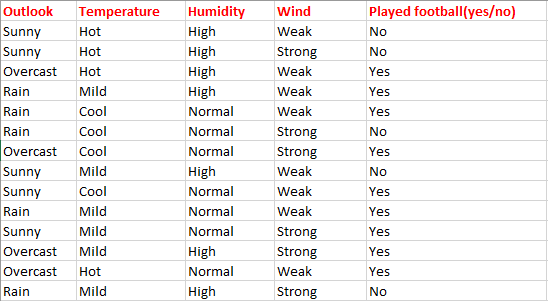
Consider the dataset shown above. It consists of 14 'points'; each point has 4 categorical attributes, and a label (yes/no).

When dealing with such categorical datasets, we may want to come up with a set of rules, or a 'protocol of questions' that will classify a new point. More concretely, we would like to come up with a tree of branching questions and decisions like this:

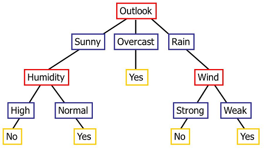
Using this tree, we could first ask about the weather 'Outlook'. If it were 'Sunny', we could then ask about the 'Humidity', and if that were 'Normal', then our decision would be 'Yes'.

This is an example of what we call a decision tree. This type of structure is called a 'tree' since if we turn it upside-down, it looks like one. Its 'leaves' are labeled with a classification decision. In this example, the classification is binary, but we can have multiple output classes as well.

Note: This is a very small example, one which does not reveal all the characteristics that are common to larger decision trees. Here, the first question attribute 'Outlook' appears only once (at the root of the tree), but other attributes could appear more than once in the tree. For example, in a larger dataset the 'Humidity' attribute could appear in many branches, and not necessarily all at the same level of the tree.

Interpretability

Decision trees are an interesting algorithm, since they have been designed to provide an explanation for each decision. This might be particularly desirable in applications such as medicine, where a physician must follow a diagnostic protocol that progressively narrows down the possibilities and issues a diagnosis (which for us is simply a 'label' for a set of features).

8.2 Which Question to Ask First? ⬤

We now want to design an algorithm that will learn a 'good' decision tree for a categorical dataset, like the 'PlayedFootball' dataset shown above. Here we will use our intuition and introduce the following learning bias: a good question is one that will allow us to gain as much information as possible about our point.

We will then need to use a measure for quantifying the information gain. The notion of entropy is known to capture information well.

8.2.1 Entropy of a Probability Distribution ⬤

Given a probability distribution $d = [p_1,\ldots,p_k]$, where $p_i\geq 0$ and $\sum_i p_i = 1$, the entropy of $p$ is defined as follows:

$$ \mathit{entropy}\,(d) = -\sum_{i=1}^k p_i \log_2 p_i \, . $$

8.2.2 Entropy of a Dataset ⬤

We now consider again our favorite dataset:

We can see that we have 9 'Yes' points and 5 'No' points. Under the assumption that each situation is equally likely, this gives a probability distribution for the labels, $[9/14, 5/14]$.

We can then define the entropy of the dataset, as the entropy of the distribution of its labels, which in this case is $- \frac{9}{14}\log_2 \frac{9}{14} - \frac{5}{14}\log_2 \frac{5}{14}$.

The smallest possible value for the entropy is 0, when one of the probabilities $p_i$ in the distribution $d$ is equal to 1. That is precisely the case when all points of the dataset will have the same label, in which case we don't even have to ask any questions!

8.2.3 Entropy of a Feature ⬤

Let's consider as an example the 'Wind' feature. This has two possible values, 'Weak' and 'Strong'. This means that the 'Wind' feature subdivides our dataset $X$ into two disjoint datasets $X_{\mathit{wind = weak}}$ and $X_{\mathit{wind = strong}}$. We can then compute the entropies of these two datasets.

$X_{\mathit{wind = weak}}$:
We have 8 days with a weak wind, and for 6 of them the answer is 'Yes'. This gives the probability distribution $d_1 = [6/8, 2/8]$, and from that we can calculate $\mathit{entropy}\,(d_1)$.

$X_{\mathit{wind = strong}}$:
We have 6 days with a strong wind, and for 3 of them the answer is 'Yes'. This gives the probability distribution $d_1 = [3/6, 3/6]$ and from that we can calculate $\mathit{entropy}\,(d_2)$.

We can then define the entropy of the 'Wind' attribute as a weighted average of these two subdataset entropies, where the weights are given by the relative sizes of the two data subsets.

$$ \mathit{entropy}\,(\mathrm{Wind}) = \frac{8}{14} \mathit{entropy}\,(d_1) + \frac{6}{14} entropy(d_2) $$

The entropy of other features can be calculated in that way. When we have a feature with $k$ values, we will calculate $k$ different entropies (for $k$ disjoint datasets) and then take their weighted average.

8.2.4 The Most Valuable Question ⬤

In order to determine the best question to ask first, we calculate the entropies of all features. The feature with the smallest entropy is the one that gives us the highest information gain.

In general, the information gain at a given node of a decision tree is taken to be the difference between the entropy at the node, and some combination of the entropies at the subtrees — typically the weighted average, but other ways can be devised.

Remark: The extreme best case occurs when asking a question will completely split our dataset into subsets where no further questions are needed (that is, subsets with entropies equal to 0).

8.3 Building the Entire Decision Tree ⬤

Given that we now have a way of finding the best question to ask for a given dataset, we can extend the idea to build an entire decision tree.

Say for example, that 'Outlook' gives us the highest information gain. This defines three disjoint datasets $X_1 = X_{\mathit{outlook=sunny}}$, $X_2 = X_{\mathit{outlook=overcast}}$ and $X_3 = X_{\mathit{outlook=rain}}$.

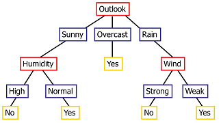
Next, we build a decision tree separately and independently for each $X_i$. That means that for each of these three data subsets, we determine the best question to ask, which will lead to further subdivisions. The process thus continues recursively. In the example image, each red box corresponds to the root a decision tree for the corresponding data subset.

When to stop asking questions: the stopping criterion

If the data subset $X'$ at some node of the tree is too small, or if its entropy is too small, then we can stop asking further questions and terminate the decision tree with a leaf. The decision issued by that leaf will be the majority class in $X'$. In the example, we see this occurring with the $X_{\mathit{outlook=overcast}}$ subset, where the entropy is 0 and the majority decision is 'Yes'.

8.4 Decision Tree Hyperparameters ⬤

Significant hyperparameters include:

• The 'information gain' criterion. There are alternative measures not based on the entropy, with the most notable being the Gini index, the default option in many implementations. The Gini index for a distribution $d=[p_1,\ldots,p_k]$ is defined as $$\mathit{gini}\,(d) = 1-\sum_{j=1}^k p_j^2\, .$$

• The 'stopping' criterion. Many stopping criteria are possible, and you can read about them in the scikit-learn documentation.

8.5 Decision Trees for Regression ⬤

Consider again a decision tree with a categorical output. As we discussed earlier, when the entropy of a data subset $X'$ is low, we can terminate the recursion with a leaf node that issues as a prediction the label of the majority of the points in $X'$.

Suppose now that the output is numerical. Although it is unlikely in practice, we can assume that the input is still categorical.

When the output is numerical, a possible analogue of the entropy is the variance for a dataset $D = (X,y)$, defined as: $$ \mathit{Var}\,(D) = \frac{1}{n} \sum_{j \in D} (y_j - E[y])^2 \, , $$ where $E[y]$ is the average of the numerical labels of the points in $D$. Intuitively, when the variance is small, all numerical labels $y$ for our dataset $D$ must fall in a very small range around $E[y]$, and thus a very simple yet effective regression model for $D$ would simply output the prediction $\hat{y} = E[y]$ for every new point $x$. When the prediction is $\hat{y} = E[y]$, the variance $\mathit{Var}(D)$ may be viewed as the mean squared error.

We can then simply replace entropy with the variance in our definitions and calculations. We can analogously define $\mathit{Var}(\mathit{feature})$, the variance with respect to each $\mathit{feature}$. Then, we can select our 'first question' to be the $\mathit{feature}$ with the smallest $\mathit{Var}(\mathit{feature})$.

As in categorical-output decision trees, the recursion can stop when a given subdataset $D'=(X',y')$ has its variance $\mathit{Var}(D')$ below some threshold, in which case the prediction will be equal to $E[y']$. Of course, alternative measures for the 'variance gain' can also be used, which accounts for one of the hyperparameters of the scikit-learn decision tree regressor .

8.6 Decision Trees for Numerical Inputs ⬤

While decision trees were originally designed for categorical features, they can also be used to handle numerical features. To do that, we convert each numerical attribute into a set of categorical features with the following discretization process.

Consider as an example attribute $x_1$. Suppose the values for $x_1$ range between two numbers $l$ and $u$ in the given dataset $X$. Then we can define a number of threshold values $\theta_1,\ldots,\theta_k$ inside the interval $[l,u]$. Then, for each data point $X_j$, we can construct $k$ binary categorical features $X'_{j,1,t}$, for $t=1\ldots, k$ as follows:

• $X'_{j,1,t} = 1$ if $X_{j,1}\geq \theta_t$
• $X'_{j,1,t} = 0$ if $X_{j,1}< \theta_t$

We can similarly define binary categorical features for each numerical feature in $X$. After doing that for all the datapoints, we will get a fully categorical feature matrix $X'$.

This process creates $k$ binary features for each original feature, which can cause some problems: the number of features can be enormous, causing the computational demands of the decision tree algorithm to explode. We can work around this problem by introducing a single feature $x'_1$ for each original feature $x_1$, but now $x'_1$ will have $k+1$ possible categorical values, equal to the number of different intervals in $[l,u]$ after partitioning by the $k$ thresholds $\theta_t$. Going back to the 'PlayedFootball' dataset, we see that its 'Wind', 'Temperature', and 'Humidity' columns most probably come from a discretization of the underlying continuous numerical features.

Comment: The values of the hyperparameters $k$ and $\theta_t$ are sometimes difficult to choose, since this requires good knowledge of the range of values for each feature. For this reason, they are often computed by special-purpose algorithms.

8.7 An Example with a Fully Numerical Dataset ⬤

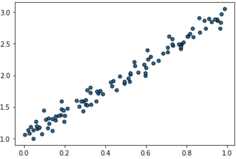
Consider now this 1-dimensional dataset, with a single numerical attribute $x$ and a numerical output $y$. As per the previous discussion, we can discretize $x$ into intervals, with a choice of thresholds such as $[0,0.1,\ldots,0.5,\ldots, 0.9, 1]$. This creates 10 binary categorical features.

For this example, it is clear that the best question to ask would be whether $x>0.5$. This is because that threshold splits the data into two parts that minimize the variance reduction criterion.

8.7 Random Forests ⬤

A random forest is a collection of $k$ random decision trees $T_1,\ldots,T_k$, where $k$ is a hyperparameter. Given a $d$ dimensional dataset of $n$ points, each of the random trees is built as follows:

• Select $n'<n$ random points from $X$. Here $n'$ is a hyperparameter, and any given point can be selected more than once (this is called random selection with replacement). Let $X'$ be the selected subset.
• Select $d'<d$ random attributes in $X'$. Here $d'$ is a hyperparameter.
• Train a decision tree on $X'$.

Given an 'ensemble' of $k$ random decision trees and a new point $x$, we classify $x$ as follows:

• Collect a list of $k$ different classifications $T_1(x),\ldots,T_k(x)$ for $x$.
• Let $c$ be the class label that appears most often in the list of $k$ classifications (in case of a tie, resolve it arbitrarily). $c$ will be the final prediction for $x$.

Comment: In a random forest, each tree may overfit to part of the dataset, but the randomness and the fact that we have multiple decision trees tends to 'cancel out' the individual overfittings. For that reason, in a random forest it is customary to not terminate the tree early, as in the case of an individual decision tree.

8.8 Decision Trees Code Notebook ⬤

Here is the scikit-learn code notebook.